Chainer Colab Notebooks : An easy way to learn and use Deep Learning
You can run notebooks on Colaboratory as soon as you can click the link of “Show on Colaboratory” of each page.
Chainer Begginer’s Hands-on
How to write a training loop in Chainer
In this notebook session we will learn how to train a deep neural network to classify hand-written digits using the popular MNIST dataset. This dataset contains 50000 training examples and 10000 test examples. Each example contains a 28x28 greyscale image and a corresponding class label for the digit. Since the digits 0-9 are used, there are 10 class labels.
Chainer provides a feature called Trainer that can be used to simplify the training process. However, we think it is good for first-time users to understand how the training process works before using the Trainer feature. Even advanced users might sometimes want to write their own training loop and so we will explain how to do so here. The complete training process consists of the following steps:
- Prepare a datasets that contain the train/validation/test examples.
- Optionally set of iterators for the datasets.
- Write a training loop that performs the following operations in each iteration:
- Retreive batches of examples from the training dataset.
- Feed the batches into the model.
- Run the forward pass on the model to compute the loss.
- Run the backward pass on the model to compute the gradients.
- Run the optimizer on the model to update the parameters.
- (Optional): Ocassionally check the performance on a validation/test set.
[2]:
# Install Chainer and CuPy!
!curl https://colab.chainer.org/install | sh -
Reading package lists... Done
Building dependency tree
Reading state information... Done
libcusparse8.0 is already the newest version (8.0.61-1).
libnvrtc8.0 is already the newest version (8.0.61-1).
libnvtoolsext1 is already the newest version (8.0.61-1).
0 upgraded, 0 newly installed, 0 to remove and 1 not upgraded.
Requirement already satisfied: cupy-cuda80==4.0.0b3 from https://github.com/kmaehashi/chainer-colab/releases/download/2018-02-06/cupy_cuda80-4.0.0b3-cp36-cp36m-linux_x86_64.whl in /usr/local/lib/python3.6/dist-packages
Requirement already satisfied: fastrlock>=0.3 in /usr/local/lib/python3.6/dist-packages (from cupy-cuda80==4.0.0b3)
Requirement already satisfied: numpy>=1.9.0 in /usr/local/lib/python3.6/dist-packages (from cupy-cuda80==4.0.0b3)
Requirement already satisfied: six>=1.9.0 in /usr/local/lib/python3.6/dist-packages (from cupy-cuda80==4.0.0b3)
Requirement already satisfied: chainer==4.0.0b3 in /usr/local/lib/python3.6/dist-packages
Requirement already satisfied: protobuf>=3.0.0 in /usr/local/lib/python3.6/dist-packages (from chainer==4.0.0b3)
Requirement already satisfied: filelock in /usr/local/lib/python3.6/dist-packages (from chainer==4.0.0b3)
Requirement already satisfied: numpy>=1.9.0 in /usr/local/lib/python3.6/dist-packages (from chainer==4.0.0b3)
Requirement already satisfied: six>=1.9.0 in /usr/local/lib/python3.6/dist-packages (from chainer==4.0.0b3)
Requirement already satisfied: setuptools in /usr/lib/python3/dist-packages (from protobuf>=3.0.0->chainer==4.0.0b3)
1. Prepare the dataset
Chainer contains some built-in functions that can be used to download and return Chainer-formated versions of popular datasets used by the ML and deep learning communities. In this example, we will use the buil-in function that retreives the MNIST dataset.
[3]:
from chainer.datasets import mnist
# Download the MNIST data if you haven't downloaded it yet
train, test = mnist.get_mnist(withlabel=True, ndim=1)
# set matplotlib so that we can see our drawing inside this notebook
%matplotlib inline
import matplotlib.pyplot as plt
# Display an example from the MNIST dataset.
# `x` contains the input image array and `t` contains that target class
# label as an integer.
x, t = train[0]
plt.imshow(x.reshape(28, 28), cmap='gray')
plt.show()
print('label:', t)
/usr/local/lib/python3.6/dist-packages/cupy/core/fusion.py:659: FutureWarning: cupy.core.fusion is experimental. The interface can change in the future.
util.experimental('cupy.core.fusion')

label: 5
2. Create the dataset iterators
Although this is an optional step, it can often be convenient to use iterators that operate on a dataset and return a certain number of examples (often called a “mini-batch”) at a time. The number of examples that is returned at a time is called the “batch size” or “mini-batch size.” Chainer already has an Iterator class and some subclasses that can be used for this purpose and it is straightforward for users to write their own as well.
We will use the SerialIterator subclass of Iterator in this example. The SerialIterator can either return the examples in the same order that they appear in the dataset (that is, in sequential order) or can shuffle the examples so that they are returned in a random order.
An Iterator can return a new minibatch by calling its ‘next()’ method. An Iterator also has properties to manage the training such as ‘epoch’: how many times we have gone through the entire dataset, ‘is_new_epoch’: whether the current iteration is the first iteration of a new epoch.
[ ]:
from chainer import iterators
# Choose the minibatch size.
batchsize = 128
train_iter = iterators.SerialIterator(train, batchsize)
test_iter = iterators.SerialIterator(test, batchsize,
repeat=False, shuffle=False)
Details about SerialIterator
SerialIteratoris a built-in subclass ofIteratorthat can be used to retrieve a dataset in either sequential or shuffled order.- The
Iteratorinitializer takes two arguments: the dataset object and a batch size. - When data need to be used repeatedly for training, set the ‘repeat’ argument to ‘True’ (the default). When data is needed only once and no longer necessary for retriving the data anymore, set ‘repeat’ to ‘False’.
- When you want to shuffle the training dataset for every epoch, set the ‘shuffle’ argument ‘True’.
In the example above, we set ‘batchsize = 128’, ‘train_iter’is the Iterator for the training dataset, and ‘test_iter’ is the Iterator for test dataset. These iterators will therefore return 128 image examples as a bundle.
3. Define the model
Now let’s define a neural network that we will train to classify the MNIST images. For simplicity, we will use a fully-connected network with three layers. We will set each hidden layer to have 100 units and set the output layer to have 10 units, corresponding to the 10 class labels for the MNIST digits 0-9.
We first briefly explain Link, Function, Chain, and Variable which are the basic components used for defining and running a model in Chainer.
Link and Function
In Chainer, each layer of a neural network is decomposed into one of two broad types of functions (actually, they are function objects): ‘Link’ and ‘Function’.
- **
Functionis a function without learnable parameters** - **
Linkis a function that contains (learnable) parameters** We can think ofLinkas wrapping aFunctionto give it parameters. That is,Linkwill contain the parameters and when it is called, it will also call a correspondingFunction.
We then describe a model by implementing code the performs the “forward pass” computations. This code will call various links and chains (recall that Link and Chain are callable objects). Chainer will take care of the “backward pass” automatically and so we do not need to worry about that unless we want to write some custom functions.
- For examples of links, see the ‘chainer.links’ module.
- For examples of functions, see the ‘chainer.functions’ module.
- For example, see the
Linearlink, which wraps thelinearfunction to give it weight and bias parameters.
Before we can start using them, we first need to import the modules as shown below.
```
import chainer.links as L
import chainer.functions as F
```
The Chainer convention is to use L for links and F for functions, like ‘L.Convolution2D(…)’ or ‘F.relu(…)’.
Chain
Chainis a class that can hold multiple links and/or functions. It is a subclass ofLinkand so it is also aLink.- This means that a chain can contain parameters, which are the parameters of any links that it deeply contains.
- In this way,
Chainallows us to construct models with a potentially deep hierarchy of functions and links. - It is often convenient to use a single chain that contains all of the layers (other chains, links, and functions) of the model. This is because we will need to optimize the model’s parameters during training and if all of the parameters are contained by a single chain, it turns out to be straightfoward to pass these parameters into an optimizer (which we describe in more detail below).
Variable
In Chainer, both the activations (that is, the inputs and outputs of function and links) and the model parameters are instances of the Variable class. A Variable holds two arrays: a data array that contains the values that are read/written during the forward pass (or the parameter values), and a grad array that contains the corresponding gradients that will are computed during the backward pass.
A Variable can potentially contain two types of arrays as well, depending whether the array resides in CPU or GPU memory. By default, the CPU is used and these will be Numpy arrays. However, it is possible to move or create these arrays on the GPU as well, in which case they will be CuPy arrays. Fortunately, CuPy uses an API that is nearly identical to Numpy. This is convinient because in addition to making it easier for users to learn (there is almost nothing to learn if you are already
familiar with Numpy), it often allows us to reuse the same code for both Numpy and CuPy arrays.
Create our model as a subclass of ‘Chain’
We can create our model to write a new subclass of Chain. The two main steps are:
- Any links (possibly also including other chains) that we wish to call during the forward computation of our chain must first be supplied to the chain’s
__init__method. After the__init__method has been called, these links will then be accessable as attributes of our chain object. This means that we also need to provide the attribute name that we want to use for each link that is supplied. We do this by providing the attribute name and corresponding link object as keyword arguments to__init__, as we will do in theMLPchain below. - We need to define a
__call__method that allows our chain to be called like a function. This method takes one or moreVariableobjects as input (that is, the input activations) and returns one or moreVariableobjects. This method executes the forward pass of the model by calling any of the links that we supplied to__init__earlier as well as any functions.
Note that the links only need to be supplied to __init__, not __call__. This is because they contain parameters. Since functions do not contain any parameters, they can be called in __call__ without having to supply them to the chain beforehand. For example, we can use a function such as F.relu by simply calling it in __call__ but a link such as L.Linear would need to first be supplied to the chain’s __init__ in order to call it in __call__.
If we decide that we want to call a link in a chain after __init__ has already been called, we can use the add_link method of Chain to add a new link at any time.
In Chainer, the Python code that implements the forward computation code itself represents the model. In other words, we can conceptually think of the computation graph for our model being constructed dynamically as this forward computation code executes. This allows Chainer to describe networks in which different computations can be performed in each iteration, such as branched networks, intuitively and with a high degree a flexibiity. This is the key feature of Chainer that we call Define-by-Run.
How to run a model on GPU
- The
LinkandChainclasses have ato_gpumethod that takes a GPU id argument specifying which GPU to use. This method sends all of the model parameters to GPU memory. - By default, the CPU is used.
[ ]:
import chainer
import chainer.links as L
import chainer.functions as F
class MLP(chainer.Chain):
def __init__(self, n_mid_units=100, n_out=10):
# register layers with parameters by super initializer
super(MLP, self).__init__()
with self.init_scope():
self.l1=L.Linear(None, n_mid_units)
self.l2=L.Linear(None, n_mid_units)
self.l3=L.Linear(None, n_out)
def __call__(self, x):
# describe the forward pass, given x (input data)
h1 = F.relu(self.l1(x))
h2 = F.relu(self.l2(h1))
return self.l3(h2)
gpu_id = 0 # change to -1 if not using GPU
model = MLP()
if gpu_id >= 0:
model.to_gpu(gpu_id)
NOTE
The L.Linear class is a link that represents a fully connected layer. When ‘None’ is passed as the first argument, this allows the number of necessary input units (n_input) and also the size of the weight and bias parameters to be automatically determined and computed at runtime during the first forward pass. We call this feature parameter shape placeholder. This can be a very helpful feature when defining deep neural network models, since it would often be tedious to manually
determine these input sizes.
As mentioned previously, a Link can contain multiple parameter arrays. For example, the L.Linear link conatins two parameter arrays: the weights W and bias b. Recall that for a given link or chain, such as the MLP chain above, the links it contains can be accessed as attributes (or properties). The parameters of a link can also be accessed as attributes. For example, following code shows how to access the bias parameter of layer l1:
[6]:
print('The shape of the bias of the first layer, l1, in the model、', model.l1.b.shape)
print('The values of the bias of the first layer in the model after initialization、', model.l1.b.data)
The shape of the bias of the first layer, l1, in the model、 (100,)
The values of the bias of the first layer in the model after initialization、 [0. 0. 0. 0. 0. 0. 0. 0. 0. 0. 0. 0. 0. 0. 0. 0. 0. 0. 0. 0. 0. 0. 0. 0.
0. 0. 0. 0. 0. 0. 0. 0. 0. 0. 0. 0. 0. 0. 0. 0. 0. 0. 0. 0. 0. 0. 0. 0.
0. 0. 0. 0. 0. 0. 0. 0. 0. 0. 0. 0. 0. 0. 0. 0. 0. 0. 0. 0. 0. 0. 0. 0.
0. 0. 0. 0. 0. 0. 0. 0. 0. 0. 0. 0. 0. 0. 0. 0. 0. 0. 0. 0. 0. 0. 0. 0.
0. 0. 0. 0.]
4. Select an optimization algorithm
Chainer provides a wide variety of optimization algorithms that can be used to optimize the model parameters during training. They are located in the chainer.optimizers module.
Here, we are going to use the basic stochastic gradient descent (SGD) method, which is implemented by optimizers.SGD. The model (recall that it is a Chain object) we created is passed to the optimizer object by providing the model as an argument to the optimizer’s ‘setup’ method. In this way, Optimizer can automatically find the model parameters to be optimized.
You can easily try out other optimizers as well. Please test and observe the results of various optimizers. For example, you could try to change ‘SGD” of ‘chainer.optimizers.SGD’ to ‘MomentumSGD’, ‘RMSprop’, ‘Adam’, etc., and run your training loop.
[ ]:
from chainer import optimizers
# Choose an optimizer algorithm
optimizer = optimizers.SGD(lr=0.01)
# Give the optimizer a reference to the model so that it
# can locate the model's parameters.
optimizer.setup(model)
NOTE
Observe that above, we setlr to 0.01 in the SGD constructor. This value is known as a the “learning rate”, one of the most important ** hyper parameters** that need be adjusted in order to obtain the best performance. The various optimizers may each have different hyper-parameters and so be sure to check the documentation for the details.
5. Write the training loop
We now show how to write the training loop. Since we are working on a digit classification problem, we will use softmax_cross_entropy as the loss function for the optimizer to minimize. For other types of problems, such as regression models, other loss functions might be more appropriate. See the Chainer documentation for detailed information on the various loss functions that are available.
Our training loop will be structured as follows. We will first get a mini-batch of examples from the training dataset. We will then feed the batch into our model by calling our model (a Chain object) like a function. This will execute the forward-pass code that we wrote for the chain’s __call__ method that we wrote above. This will cause the model to output class label predictions that we supply to the loss function along with the true (that is, target) values. The loss function will
output the loss as a Variable object. We then clear any previous gradients and perform the backward pass by calling the backward method on the loss variable which computes the parameter gradients. We need to clear the gradients first because the backward method accumulates gradients instead of overwriting the previous values. Since the optimizer already was given a reference to the model, it already has access to the parameters and the newly-computed gradients and so we can now call
the update method of the optimizer which will update the model parameters.
At this point you might be wondering how calling backward on the loss variable could possibly compute the gradients for all of the model parameters. This works as follows. First recall that all activation and parameter arrays in the model are instances of Variable. During the forward pass, as each function is called on its inputs, we save references in each output variable that refer to the function that created it and its input variables. In this way, by the time the final loss variable
is computed, it actually contains backward references that lead all the way back to the input variables of the model. That is, the loss variable contains a representation of the entire computational graph of the model, which is recomputed each time the forward pass is performed. By following these backward references from the loss variable, each function as a backward method that gets called to compute any parameter gradients. Thus, by the time the end of the backward graph is reached (at
the input variables of the model), all parameter gradients have been computed.
Thus, there are four steps in single training loop iteration as shown below.
- Obtain and pass a mini-batch of example images into the model and obtain the output digit predictions
prediction_train. - Compute the loss function, giving it the predicted labels from the output of our model and also the true “target” label values.
- Clear any previous gradients and call the backward method of ‘Variable’ to compute the parameter gradients for the model.
- Call the ‘update’ method of Optimizer, which performs one optimization step and updates all of the model parameters.
In addition to the above steps, it is good to occasionally check the performance of our model on a validation and/or test set. This allows us to observe how well it can generalize to new data and also check whether it is overfitting. The code below checks the performance on the test set at the end of each epoch. The code has the same structure as the training code except that no backpropagation is performed and we also commpute the accuracy on the test set using the F.accuracy function.
We can write the training loop code as follows:
[8]:
import numpy as np
from chainer.dataset import concat_examples
from chainer.cuda import to_cpu
max_epoch = 10
while train_iter.epoch < max_epoch:
# ---------- The first iteration of training loop ----------
train_batch = train_iter.next()
image_train, target_train = concat_examples(train_batch, gpu_id)
# calculate the prediction of the model
prediction_train = model(image_train)
# calculation of loss function, softmax_cross_entropy
loss = F.softmax_cross_entropy(prediction_train, target_train)
# calculate the gradients in the model
model.cleargrads()
loss.backward()
# update the parameters of the model
optimizer.update()
# --------------- until here One loop ----------------
# Check if the generalization of the model is improving
# by measuring the accuracy of prediction after every epoch
if train_iter.is_new_epoch: # after finishing the first epoch
# display the result of the loss function
print('epoch:{:02d} train_loss:{:.04f} '.format(
train_iter.epoch, float(to_cpu(loss.data))), end='')
test_losses = []
test_accuracies = []
for test_batch in test_iter:
test_batch = test_iter.next()
image_test, target_test = concat_examples(test_batch, gpu_id)
# forward the test data
prediction_test = model(image_test)
# calculate the loss function
loss_test = F.softmax_cross_entropy(prediction_test, target_test)
test_losses.append(to_cpu(loss_test.data))
# calculate the accuracy
accuracy = F.accuracy(prediction_test, target_test)
accuracy.to_cpu()
test_accuracies.append(accuracy.data)
test_iter.reset()
print('val_loss:{:.04f} val_accuracy:{:.04f}'.format(
np.mean(test_losses), np.mean(test_accuracies)))
epoch:01 train_loss:0.9583 val_loss:0.7864 val_accuracy:0.8211
epoch:02 train_loss:0.4803 val_loss:0.4501 val_accuracy:0.8812
epoch:03 train_loss:0.3057 val_loss:0.3667 val_accuracy:0.8982
epoch:04 train_loss:0.2477 val_loss:0.3292 val_accuracy:0.9054
epoch:05 train_loss:0.2172 val_loss:0.3059 val_accuracy:0.9133
epoch:06 train_loss:0.2202 val_loss:0.2880 val_accuracy:0.9176
epoch:07 train_loss:0.3009 val_loss:0.2758 val_accuracy:0.9214
epoch:08 train_loss:0.3399 val_loss:0.2632 val_accuracy:0.9252
epoch:09 train_loss:0.3497 val_loss:0.2538 val_accuracy:0.9287
epoch:10 train_loss:0.1691 val_loss:0.2430 val_accuracy:0.9311
6. Save the trained model
Chainer provides two types of serializers that can be used to save and restore model state. One supports the HDF5 format and the other supports the Numpy NPZ format. For this example, we are going to use the NPZ format to save our model since it is easy to use with Numpy without requiring an additional dependencies or libraries.
[9]:
from chainer import serializers
serializers.save_npz('my_mnist.model', model)
# check if the model is saved.
%ls -la my_mnist.model
-rw-r--r-- 1 root root 333954 Feb 23 08:13 my_mnist.model
7. Perform classification by restoring a previously trained model
We will now use our previously trained and saved MNIST model to classify a new image. In order to load a previously-trained model, we need to perform the following two steps: 1. We must use the same model definition code the was used to create the previously-trained model. For our example, this is the MLP chain that we created earlier. 2. We then overwrite any parameters in the newly-created model with the values that were saved earlier using the serializer. The serializers.load_npz
function can be used to do this.
Now that the model has been restored, it can be used to predict image labels on new input images.
[ ]:
# Create the infrence (evaluation) model as the previous model
infer_model = MLP()
# Load the saved parameters into the parameters of the new inference model to overwrite
serializers.load_npz('my_mnist.model', infer_model)
# Send the model to utilize GPU by to_GPU
if gpu_id >= 0:
infer_model.to_gpu(gpu_id)
[11]:
# Get a test image and label
x, t = test[0]
plt.imshow(x.reshape(28, 28), cmap='gray')
plt.show()
print('label:', t)

label: 7
[12]:
from chainer.cuda import to_gpu
# change the shape to minibutch.
# In this example, the size of minibatch is 1.
# Inference using any mini-batch size can be performed.
print(x.shape, end=' -> ')
x = x[None, ...]
print(x.shape)
# to calculate by GPU, send the data to GPU, too.
if gpu_id >= 0:
x = to_gpu(x, 0)
# forward calculation of the model by sending X
y = infer_model(x)
# The result is given as Variable, then we can take a look at the contents by the attribute, .data.
y = y.data
# send the gpu result to cpu
y = to_cpu(y)
# The most probable number by looking at the argmax
pred_label = y.argmax(axis=1)
print('predicted label:', pred_label[0])
(784,) -> (1, 784)
predicted label: 7
Using the Trainer feature
Chainer has a feature called Trainer that can often be used to simplify the process of training and evaluating a model. This feature supports training a model in a way such that the user is not required to explicitly write the code for the training loop. For many types of models, including our MNIST model, Trainer allows us to write our training and evaluation code much more concisely.
Chainer contains several extensions that can be used with Trainer to visualize your results, evaluate your model, store and manage log files more easily.
This example will show how to use the Trainer feature to train a fully-connected feed-forward neural network on the MNIST dataset.
[1]:
# Install Chainer and CuPy!
!curl https://colab.chainer.org/install | sh -
Reading package lists... Done
Building dependency tree
Reading state information... Done
libcusparse8.0 is already the newest version (8.0.61-1).
libnvrtc8.0 is already the newest version (8.0.61-1).
libnvtoolsext1 is already the newest version (8.0.61-1).
0 upgraded, 0 newly installed, 0 to remove and 1 not upgraded.
Requirement already satisfied: cupy-cuda80==4.0.0b3 from https://github.com/kmaehashi/chainer-colab/releases/download/2018-02-06/cupy_cuda80-4.0.0b3-cp36-cp36m-linux_x86_64.whl in /usr/local/lib/python3.6/dist-packages
Requirement already satisfied: fastrlock>=0.3 in /usr/local/lib/python3.6/dist-packages (from cupy-cuda80==4.0.0b3)
Requirement already satisfied: numpy>=1.9.0 in /usr/local/lib/python3.6/dist-packages (from cupy-cuda80==4.0.0b3)
Requirement already satisfied: six>=1.9.0 in /usr/local/lib/python3.6/dist-packages (from cupy-cuda80==4.0.0b3)
Requirement already satisfied: chainer==4.0.0b3 in /usr/local/lib/python3.6/dist-packages
Requirement already satisfied: protobuf>=3.0.0 in /usr/local/lib/python3.6/dist-packages (from chainer==4.0.0b3)
Requirement already satisfied: numpy>=1.9.0 in /usr/local/lib/python3.6/dist-packages (from chainer==4.0.0b3)
Requirement already satisfied: filelock in /usr/local/lib/python3.6/dist-packages (from chainer==4.0.0b3)
Requirement already satisfied: six>=1.9.0 in /usr/local/lib/python3.6/dist-packages (from chainer==4.0.0b3)
Requirement already satisfied: setuptools in /usr/lib/python3/dist-packages (from protobuf>=3.0.0->chainer==4.0.0b3)
1. Prepare the dataset
Load the MNIST dataset, as in the previous notebook.
[2]:
from chainer.datasets import mnist
train, test = mnist.get_mnist()
/usr/local/lib/python3.6/dist-packages/cupy/core/fusion.py:659: FutureWarning: cupy.core.fusion is experimental. The interface can change in the future.
util.experimental('cupy.core.fusion')
Downloading from http://yann.lecun.com/exdb/mnist/train-images-idx3-ubyte.gz...
Downloading from http://yann.lecun.com/exdb/mnist/train-labels-idx1-ubyte.gz...
Downloading from http://yann.lecun.com/exdb/mnist/t10k-images-idx3-ubyte.gz...
Downloading from http://yann.lecun.com/exdb/mnist/t10k-labels-idx1-ubyte.gz...
2. Prepare the dataset iterators
[ ]:
from chainer import iterators
batchsize = 128
train_iter = iterators.SerialIterator(train, batchsize)
test_iter = iterators.SerialIterator(test, batchsize, False, False)
3. Prepare the Model
We use the same model as before.
[ ]:
import chainer
import chainer.links as L
import chainer.functions as F
class MLP(chainer.Chain):
def __init__(self, n_mid_units=100, n_out=10):
super(MLP, self).__init__()
with self.init_scope():
self.l1=L.Linear(None, n_mid_units)
self.l2=L.Linear(None, n_mid_units)
self.l3=L.Linear(None, n_out)
def __call__(self, x):
h1 = F.relu(self.l1(x))
h2 = F.relu(self.l2(h1))
return self.l3(h2)
gpu_id = 0 # Set to -1 if you don't have a GPU
model = MLP()
if gpu_id >= 0:
model.to_gpu(gpu_id)
4. Prepare the Updater
As mentioned above, the trainer object (instance of Trainer) actually implements the training loop for us. However, before we can use it, we must first prepare another object that will actually perform one iteration of training operations and pass it to the trainer. This other object will be an subclass of Updater such as StandardUpdater or a custom subclass. It will therefore need to hold all of the components that are needed in order to perform one iteration of training, such as a
dataset iterator, and optimizer that also holds the model.
- Updater
- Iterator
- Dataset
- Optimizer
- Model
- Iterator
Since we can also write customized updaters, they can perform any kinds of computations. However, for this example we will use the StandardUpdater which performs the following steps each time it is called:
- Retrieve a batch of data from a dataset using the iterator that we supplied.
- Feed the batch into the model and calculate the loss using the optimizer that we supplied. Since we will supply the model to the optimizer first, this means that the updater can also access the model from the optimizer.
- Update the model parameters using the optimizer that we supplied.
Once the updater has been set up, we can pass it to the trainer and start the training process. The trainer will then automatically create the training loop and call the updater once per iteration.
Now let’s create the updater object.
[ ]:
from chainer import optimizers
from chainer import training
max_epoch = 10
# Note: L.Classifier is actually a chain that wraps 'model' to add a loss
# function.
# Since we do not specify a loss funciton here, the default
# 'softmax_cross_entropy' is used.
# The output of this modified 'model' will now be a loss value instead
# of a class label prediction.
model = L.Classifier(model)
# Send the model to the GPU.
if gpu_id >= 0:
model.to_gpu(gpu_id)
# selection of your optimizing method
optimizer = optimizers.SGD()
# Give the optimizer a reference to the model
optimizer.setup(model)
# Get an Updater that uses the Iterator and Optimizer
updater = training.StandardUpdater(train_iter, optimizer, device=gpu_id)
NOTE
The L.Classifier object is actually a chain that places our model in its predictor attribute. This modifies model so that when it is called, it will now take both the input image batch and a class label batch as inputs to its __call__ method and output a Variable that contains the loss value. The loss function to use can be optionally set but we use the default which is softmax_cross_entropy.
Specifically, when __call__ is called on our model (which is now a L.Classifier object), the image batch is supplied to its predictor attribute, which contains our MLP model. The ourput of the MLP (which consists of class label predictions) is supplied to the loss function along with the target class labels to compute the loss value which is then returned as a Variable object.
Note that we use StandardUpdater, which is the simplest type of Updater in Chainer. There are also other types of updaters available, such as ParallelUpdater (which is intended for multiple GPUs) and you can also write a custom updater if you wish.
5. Setup Trainer
Now that we have set up an updater, we can pass it to a Trainer object. You can optionally pass a stop_trigger to the second trainer argument as a tuple, (length, unit) to tell the trainer stop automatically according to your indicated timing. The length is given as an arbitrary integer and unit is given as a string which currently must be either epoch or iteration. Without setting stop_trigger, the training will not stop automatically.
[ ]:
# Send Updater to Trainer
trainer = training.Trainer(updater, (max_epoch, 'epoch'),
out='mnist_result')
The out argument in the trainer will set up an output directory to save the logfiles, the image files of graphs to show the time progress of loss, accuracy, etc.
Next, we will explain how to display/save those outputs by using extensions.
6. Add extensions to trainer
There are several optional trainer extensions that provide the following capabilites:
- Save log files automatically (
LogReport) - Display the training information to the terminal periodically (
PrintReport) - Visualize the loss progress by plottig a graph periodically and save its image (
PlotReport) - Automatically serialize the model or the state of Optimizer periodically (
snapshot/snapshot_object) - Display Progress Bar to show the progress of training (
ProgressBar) - Save the model architecture as a dot format readable by
Graphviz(dump_graph)
Now you can utilize the wide variety of tools shown above right away! To do so, simply pass the desired extensions object to the Trainer object by using the extend() method of Trainer.
[ ]:
from chainer.training import extensions
trainer.extend(extensions.LogReport())
trainer.extend(extensions.PrintReport(['epoch', 'main/loss', 'main/accuracy', 'validation/main/loss', 'validation/main/accuracy', 'elapsed_time']))
trainer.extend(extensions.PlotReport(['main/loss', 'validation/main/loss'], x_key='epoch', file_name='loss.png'))
trainer.extend(extensions.PlotReport(['main/accuracy', 'validation/main/accuracy'], x_key='epoch', file_name='accuracy.png'))
trainer.extend(extensions.snapshot(filename='snapshot_epoch-{.updater.epoch}'))
trainer.extend(extensions.snapshot_object(model.predictor, filename='model_epoch-{.updater.epoch}'))
trainer.extend(extensions.Evaluator(test_iter, model, device=gpu_id))
trainer.extend(extensions.dump_graph('main/loss'))
LogReport
Collect loss and accuracy automatically every epoch or iteration and store the information under the log file in the directory assigned by the out argument of Trainer.
PrintReport
Reporter aggregates the results to output to the standard output. The timing for displaying the output can be given by the list.
PlotReport
PlotReport plots the values specified by its arguments, draws the graph and saves the image in the directory set by ‘file name’.
snapshot
The snapshot method saves the Trainer object at the designated timing (defaut: every epoch) in the directory assigned by out argument in Trainer. The Trainer object, as mentioned before, has an Updater which contains an Optimizer and a model inside. Therefore, as long as you have the snapshot file, you can use it to come back to the training or make inferences using the previously trained model later.
snapshot_object
When you save the whole Trainer object, in some cases it is very tedious to retrieve only the inside of the model. By using snapshot_object, you can save the particular object (in this case, the model wrapped by Classifier) in addition to saving the Trainer object. Classifier is a Chain object that keeps the Chain object given by the first argument as a property called predictor and calculates the loss. Classifier doesn’t have any parameters other than those
inside its predictor model, and so we only save model.predictor.
Evaluator
The Iterator that uses the evaluation dataset (such as a validation or test dataset) and the model object are passed to Evaluator. The Evaluator evaluates the model using the given dataset at the specified timing interval.
dump_graph
This method saves the computational graph of the model. The graph is saved in Graphviz dot format. The output location (directory) to save the graph is set by the out argument of Trainer.
The extensions class has a lot of options other than those mentioned here. For instance, by using the trigger option, you can set individual timings to activate the extensions more flexibly. Please take a look at the official document in more detail:Trainer extensions
7. Start Training
To start training, just call run method from Trainer object.
[8]:
trainer.run()
epoch main/loss main/accuracy validation/main/loss validation/main/accuracy elapsed_time
1 1.59174 0.605827 0.830716 0.811017 11.9659
2 0.620236 0.8436 0.468635 0.878362 15.3477
3 0.434218 0.883229 0.375343 0.897943 18.6432
4 0.370276 0.896985 0.331921 0.906843 21.9966
5 0.336392 0.905517 0.306286 0.914062 25.3211
6 0.313135 0.911114 0.290228 0.917623 28.6711
7 0.296385 0.915695 0.277794 0.921084 32.0399
8 0.282124 0.919338 0.264538 0.924248 35.3713
9 0.269923 0.922858 0.257158 0.923853 38.7191
10 0.25937 0.925373 0.245689 0.927907 42.0867
Let’s see the graph of loss saved in the mnist_result directory.
[9]:
from IPython.display import Image
Image(filename='mnist_result/loss.png')
[9]:

How about the accuracy?
[10]:
Image(filename='mnist_result/accuracy.png')
[10]:

Furthermore, let’s visualize the computational graph output by dump_graph of extensions using Graphviz.
[13]:
!apt-get install graphviz -y
!dot -Tpng mnist_result/cg.dot -o mnist_result/cg.png
Reading package lists... Done
Building dependency tree
Reading state information... Done
The following additional packages will be installed:
fontconfig libcairo2 libcdt5 libcgraph6 libdatrie1 libgd3 libgraphite2-3
libgvc6 libgvpr2 libharfbuzz0b libice6 libjbig0 libltdl7 libpango-1.0-0
libpangocairo-1.0-0 libpangoft2-1.0-0 libpathplan4 libpixman-1-0 libsm6
libthai-data libthai0 libtiff5 libwebp6 libxaw7 libxcb-render0 libxcb-shm0
libxext6 libxmu6 libxpm4 libxt6 x11-common
Suggested packages:
gsfonts graphviz-doc libgd-tools
The following NEW packages will be installed:
fontconfig graphviz libcairo2 libcdt5 libcgraph6 libdatrie1 libgd3
libgraphite2-3 libgvc6 libgvpr2 libharfbuzz0b libice6 libjbig0 libltdl7
libpango-1.0-0 libpangocairo-1.0-0 libpangoft2-1.0-0 libpathplan4
libpixman-1-0 libsm6 libthai-data libthai0 libtiff5 libwebp6 libxaw7
libxcb-render0 libxcb-shm0 libxext6 libxmu6 libxpm4 libxt6 x11-common
0 upgraded, 32 newly installed, 0 to remove and 1 not upgraded.
Need to get 4,228 kB of archives.
After this operation, 21.2 MB of additional disk space will be used.
Get:1 http://archive.ubuntu.com/ubuntu artful/main amd64 libxext6 amd64 2:1.3.3-1 [29.4 kB]
Get:2 http://archive.ubuntu.com/ubuntu artful/main amd64 fontconfig amd64 2.11.94-0ubuntu2 [177 kB]
Get:3 http://archive.ubuntu.com/ubuntu artful/main amd64 x11-common all 1:7.7+19ubuntu3 [22.0 kB]
Get:4 http://archive.ubuntu.com/ubuntu artful/main amd64 libice6 amd64 2:1.0.9-2 [40.2 kB]
Get:5 http://archive.ubuntu.com/ubuntu artful/main amd64 libsm6 amd64 2:1.2.2-1 [15.8 kB]
Get:6 http://archive.ubuntu.com/ubuntu artful/main amd64 libjbig0 amd64 2.1-3.1 [26.6 kB]
Get:7 http://archive.ubuntu.com/ubuntu artful/main amd64 libcdt5 amd64 2.38.0-16ubuntu2 [19.5 kB]
Get:8 http://archive.ubuntu.com/ubuntu artful/main amd64 libcgraph6 amd64 2.38.0-16ubuntu2 [40.0 kB]
Get:9 http://archive.ubuntu.com/ubuntu artful/main amd64 libtiff5 amd64 4.0.8-5 [150 kB]
Get:10 http://archive.ubuntu.com/ubuntu artful/main amd64 libwebp6 amd64 0.6.0-3 [181 kB]
Get:11 http://archive.ubuntu.com/ubuntu artful/main amd64 libxpm4 amd64 1:3.5.12-1 [34.0 kB]
Get:12 http://archive.ubuntu.com/ubuntu artful/main amd64 libgd3 amd64 2.2.5-3 [119 kB]
Get:13 http://archive.ubuntu.com/ubuntu artful/main amd64 libpixman-1-0 amd64 0.34.0-1 [230 kB]
Get:14 http://archive.ubuntu.com/ubuntu artful/main amd64 libxcb-render0 amd64 1.12-1ubuntu1 [14.8 kB]
Get:15 http://archive.ubuntu.com/ubuntu artful/main amd64 libxcb-shm0 amd64 1.12-1ubuntu1 [5,482 B]
Get:16 http://archive.ubuntu.com/ubuntu artful/main amd64 libcairo2 amd64 1.14.10-1ubuntu1 [558 kB]
Get:17 http://archive.ubuntu.com/ubuntu artful/main amd64 libltdl7 amd64 2.4.6-2 [38.8 kB]
Get:18 http://archive.ubuntu.com/ubuntu artful/main amd64 libthai-data all 0.1.26-3 [132 kB]
Get:19 http://archive.ubuntu.com/ubuntu artful/main amd64 libdatrie1 amd64 0.2.10-5 [17.6 kB]
Get:20 http://archive.ubuntu.com/ubuntu artful/main amd64 libthai0 amd64 0.1.26-3 [17.7 kB]
Get:21 http://archive.ubuntu.com/ubuntu artful/main amd64 libpango-1.0-0 amd64 1.40.12-1 [152 kB]
Get:22 http://archive.ubuntu.com/ubuntu artful/main amd64 libgraphite2-3 amd64 1.3.10-2 [78.3 kB]
Get:23 http://archive.ubuntu.com/ubuntu artful/main amd64 libharfbuzz0b amd64 1.4.2-1 [211 kB]
Get:24 http://archive.ubuntu.com/ubuntu artful/main amd64 libpangoft2-1.0-0 amd64 1.40.12-1 [33.2 kB]
Get:25 http://archive.ubuntu.com/ubuntu artful/main amd64 libpangocairo-1.0-0 amd64 1.40.12-1 [20.8 kB]
Get:26 http://archive.ubuntu.com/ubuntu artful/main amd64 libpathplan4 amd64 2.38.0-16ubuntu2 [22.6 kB]
Get:27 http://archive.ubuntu.com/ubuntu artful/main amd64 libgvc6 amd64 2.38.0-16ubuntu2 [587 kB]
Get:28 http://archive.ubuntu.com/ubuntu artful/main amd64 libgvpr2 amd64 2.38.0-16ubuntu2 [167 kB]
Get:29 http://archive.ubuntu.com/ubuntu artful/main amd64 libxt6 amd64 1:1.1.5-1 [160 kB]
Get:30 http://archive.ubuntu.com/ubuntu artful/main amd64 libxmu6 amd64 2:1.1.2-2 [46.0 kB]
Get:31 http://archive.ubuntu.com/ubuntu artful/main amd64 libxaw7 amd64 2:1.0.13-1 [173 kB]
Get:32 http://archive.ubuntu.com/ubuntu artful/main amd64 graphviz amd64 2.38.0-16ubuntu2 [710 kB]
Fetched 4,228 kB in 4s (954 kB/s)
Extracting templates from packages: 100%
Selecting previously unselected package libxext6:amd64.
(Reading database ... 16692 files and directories currently installed.)
Preparing to unpack .../00-libxext6_2%3a1.3.3-1_amd64.deb ...
Unpacking libxext6:amd64 (2:1.3.3-1) ...
Selecting previously unselected package fontconfig.
Preparing to unpack .../01-fontconfig_2.11.94-0ubuntu2_amd64.deb ...
Unpacking fontconfig (2.11.94-0ubuntu2) ...
Selecting previously unselected package x11-common.
Preparing to unpack .../02-x11-common_1%3a7.7+19ubuntu3_all.deb ...
Unpacking x11-common (1:7.7+19ubuntu3) ...
Selecting previously unselected package libice6:amd64.
Preparing to unpack .../03-libice6_2%3a1.0.9-2_amd64.deb ...
Unpacking libice6:amd64 (2:1.0.9-2) ...
Selecting previously unselected package libsm6:amd64.
Preparing to unpack .../04-libsm6_2%3a1.2.2-1_amd64.deb ...
Unpacking libsm6:amd64 (2:1.2.2-1) ...
Selecting previously unselected package libjbig0:amd64.
Preparing to unpack .../05-libjbig0_2.1-3.1_amd64.deb ...
Unpacking libjbig0:amd64 (2.1-3.1) ...
Selecting previously unselected package libcdt5.
Preparing to unpack .../06-libcdt5_2.38.0-16ubuntu2_amd64.deb ...
Unpacking libcdt5 (2.38.0-16ubuntu2) ...
Selecting previously unselected package libcgraph6.
Preparing to unpack .../07-libcgraph6_2.38.0-16ubuntu2_amd64.deb ...
Unpacking libcgraph6 (2.38.0-16ubuntu2) ...
Selecting previously unselected package libtiff5:amd64.
Preparing to unpack .../08-libtiff5_4.0.8-5_amd64.deb ...
Unpacking libtiff5:amd64 (4.0.8-5) ...
Selecting previously unselected package libwebp6:amd64.
Preparing to unpack .../09-libwebp6_0.6.0-3_amd64.deb ...
Unpacking libwebp6:amd64 (0.6.0-3) ...
Selecting previously unselected package libxpm4:amd64.
Preparing to unpack .../10-libxpm4_1%3a3.5.12-1_amd64.deb ...
Unpacking libxpm4:amd64 (1:3.5.12-1) ...
Selecting previously unselected package libgd3:amd64.
Preparing to unpack .../11-libgd3_2.2.5-3_amd64.deb ...
Unpacking libgd3:amd64 (2.2.5-3) ...
Selecting previously unselected package libpixman-1-0:amd64.
Preparing to unpack .../12-libpixman-1-0_0.34.0-1_amd64.deb ...
Unpacking libpixman-1-0:amd64 (0.34.0-1) ...
Selecting previously unselected package libxcb-render0:amd64.
Preparing to unpack .../13-libxcb-render0_1.12-1ubuntu1_amd64.deb ...
Unpacking libxcb-render0:amd64 (1.12-1ubuntu1) ...
Selecting previously unselected package libxcb-shm0:amd64.
Preparing to unpack .../14-libxcb-shm0_1.12-1ubuntu1_amd64.deb ...
Unpacking libxcb-shm0:amd64 (1.12-1ubuntu1) ...
Selecting previously unselected package libcairo2:amd64.
Preparing to unpack .../15-libcairo2_1.14.10-1ubuntu1_amd64.deb ...
Unpacking libcairo2:amd64 (1.14.10-1ubuntu1) ...
Selecting previously unselected package libltdl7:amd64.
Preparing to unpack .../16-libltdl7_2.4.6-2_amd64.deb ...
Unpacking libltdl7:amd64 (2.4.6-2) ...
Selecting previously unselected package libthai-data.
Preparing to unpack .../17-libthai-data_0.1.26-3_all.deb ...
Unpacking libthai-data (0.1.26-3) ...
Selecting previously unselected package libdatrie1:amd64.
Preparing to unpack .../18-libdatrie1_0.2.10-5_amd64.deb ...
Unpacking libdatrie1:amd64 (0.2.10-5) ...
Selecting previously unselected package libthai0:amd64.
Preparing to unpack .../19-libthai0_0.1.26-3_amd64.deb ...
Unpacking libthai0:amd64 (0.1.26-3) ...
Selecting previously unselected package libpango-1.0-0:amd64.
Preparing to unpack .../20-libpango-1.0-0_1.40.12-1_amd64.deb ...
Unpacking libpango-1.0-0:amd64 (1.40.12-1) ...
Selecting previously unselected package libgraphite2-3:amd64.
Preparing to unpack .../21-libgraphite2-3_1.3.10-2_amd64.deb ...
Unpacking libgraphite2-3:amd64 (1.3.10-2) ...
Selecting previously unselected package libharfbuzz0b:amd64.
Preparing to unpack .../22-libharfbuzz0b_1.4.2-1_amd64.deb ...
Unpacking libharfbuzz0b:amd64 (1.4.2-1) ...
Selecting previously unselected package libpangoft2-1.0-0:amd64.
Preparing to unpack .../23-libpangoft2-1.0-0_1.40.12-1_amd64.deb ...
Unpacking libpangoft2-1.0-0:amd64 (1.40.12-1) ...
Selecting previously unselected package libpangocairo-1.0-0:amd64.
Preparing to unpack .../24-libpangocairo-1.0-0_1.40.12-1_amd64.deb ...
Unpacking libpangocairo-1.0-0:amd64 (1.40.12-1) ...
Selecting previously unselected package libpathplan4.
Preparing to unpack .../25-libpathplan4_2.38.0-16ubuntu2_amd64.deb ...
Unpacking libpathplan4 (2.38.0-16ubuntu2) ...
Selecting previously unselected package libgvc6.
Preparing to unpack .../26-libgvc6_2.38.0-16ubuntu2_amd64.deb ...
Unpacking libgvc6 (2.38.0-16ubuntu2) ...
Selecting previously unselected package libgvpr2.
Preparing to unpack .../27-libgvpr2_2.38.0-16ubuntu2_amd64.deb ...
Unpacking libgvpr2 (2.38.0-16ubuntu2) ...
Selecting previously unselected package libxt6:amd64.
Preparing to unpack .../28-libxt6_1%3a1.1.5-1_amd64.deb ...
Unpacking libxt6:amd64 (1:1.1.5-1) ...
Selecting previously unselected package libxmu6:amd64.
Preparing to unpack .../29-libxmu6_2%3a1.1.2-2_amd64.deb ...
Unpacking libxmu6:amd64 (2:1.1.2-2) ...
Selecting previously unselected package libxaw7:amd64.
Preparing to unpack .../30-libxaw7_2%3a1.0.13-1_amd64.deb ...
Unpacking libxaw7:amd64 (2:1.0.13-1) ...
Selecting previously unselected package graphviz.
Preparing to unpack .../31-graphviz_2.38.0-16ubuntu2_amd64.deb ...
Unpacking graphviz (2.38.0-16ubuntu2) ...
Setting up libpathplan4 (2.38.0-16ubuntu2) ...
Setting up libxcb-render0:amd64 (1.12-1ubuntu1) ...
Setting up libxext6:amd64 (2:1.3.3-1) ...
Setting up libjbig0:amd64 (2.1-3.1) ...
Setting up libdatrie1:amd64 (0.2.10-5) ...
Setting up libtiff5:amd64 (4.0.8-5) ...
Setting up libgraphite2-3:amd64 (1.3.10-2) ...
Setting up libpixman-1-0:amd64 (0.34.0-1) ...
Processing triggers for libc-bin (2.26-0ubuntu2.1) ...
Setting up libltdl7:amd64 (2.4.6-2) ...
Setting up libxcb-shm0:amd64 (1.12-1ubuntu1) ...
Setting up libxpm4:amd64 (1:3.5.12-1) ...
Setting up libthai-data (0.1.26-3) ...
Setting up x11-common (1:7.7+19ubuntu3) ...
update-rc.d: warning: start and stop actions are no longer supported; falling back to defaults
invoke-rc.d: could not determine current runlevel
invoke-rc.d: policy-rc.d denied execution of start.
Setting up libcdt5 (2.38.0-16ubuntu2) ...
Setting up fontconfig (2.11.94-0ubuntu2) ...
Regenerating fonts cache... done.
Setting up libcgraph6 (2.38.0-16ubuntu2) ...
Setting up libwebp6:amd64 (0.6.0-3) ...
Setting up libcairo2:amd64 (1.14.10-1ubuntu1) ...
Setting up libgvpr2 (2.38.0-16ubuntu2) ...
Setting up libgd3:amd64 (2.2.5-3) ...
Setting up libharfbuzz0b:amd64 (1.4.2-1) ...
Setting up libthai0:amd64 (0.1.26-3) ...
Setting up libpango-1.0-0:amd64 (1.40.12-1) ...
Setting up libice6:amd64 (2:1.0.9-2) ...
Setting up libsm6:amd64 (2:1.2.2-1) ...
Setting up libpangoft2-1.0-0:amd64 (1.40.12-1) ...
Setting up libxt6:amd64 (1:1.1.5-1) ...
Setting up libpangocairo-1.0-0:amd64 (1.40.12-1) ...
Setting up libxmu6:amd64 (2:1.1.2-2) ...
Setting up libxaw7:amd64 (2:1.0.13-1) ...
Setting up libgvc6 (2.38.0-16ubuntu2) ...
Setting up graphviz (2.38.0-16ubuntu2) ...
Processing triggers for libc-bin (2.26-0ubuntu2.1) ...
[14]:
Image(filename='mnist_result/cg.png')
[14]:

From the top to the bottom, you can track the data flow of the computations, how data and parameters are passed to what type of Function and the calculated loss is output.
8. Evaluate a pre-trained model
[15]:
import numpy as np
from chainer import serializers
from chainer.cuda import to_gpu
from chainer.cuda import to_cpu
model = MLP()
serializers.load_npz('mnist_result/model_epoch-10', model)
%matplotlib inline
import matplotlib.pyplot as plt
x, t = test[0]
plt.imshow(x.reshape(28, 28), cmap='gray')
plt.show()
print('label:', t)
if gpu_id >= 0:
model.to_gpu(gpu_id)
x = to_gpu(x[None, ...])
y = model(x)
y = to_cpu(y.data)
else:
x = x[None, ...]
y = model(x)
y = y.data
print('predicted_label:', y.argmax(axis=1)[0])

label: 7
predicted_label: 7
It successfully executed !!
Creating and training convolutional neural networks
We will now improve upon our previous example by creating some more sophisticed image classifiers and using a more challanging dataset. Specifically, we will implement convolutional neural networks (CNNs) and train them using the CIFAR10 dataset, which uses natural color images. This dataset uses 60000 small color images of size 32x32x3 (the 3 is for the RGB color channels) and 10 class labels. 50000 of these are used for training and the remaining 10000 are for the test set. There is also a CIFAR100 version that uses 100 class labels, but we will only use CIFAR10 here.
| airplane | automobile | bird | cat | deer | dog | frog | horse | ship | truck |
|---|---|---|---|---|---|---|---|---|---|
 |
 |
 |
 |
 |
 |
 |
 |
 |
 |
[2]:
# Install Chainer and CuPy!
!curl https://colab.chainer.org/install | sh -
Reading package lists... Done
Building dependency tree
Reading state information... Done
libcusparse8.0 is already the newest version (8.0.61-1).
libnvrtc8.0 is already the newest version (8.0.61-1).
libnvtoolsext1 is already the newest version (8.0.61-1).
0 upgraded, 0 newly installed, 0 to remove and 1 not upgraded.
Requirement already satisfied: cupy-cuda80==4.0.0b3 from https://github.com/kmaehashi/chainer-colab/releases/download/2018-02-06/cupy_cuda80-4.0.0b3-cp36-cp36m-linux_x86_64.whl in /usr/local/lib/python3.6/dist-packages
Requirement already satisfied: fastrlock>=0.3 in /usr/local/lib/python3.6/dist-packages (from cupy-cuda80==4.0.0b3)
Requirement already satisfied: numpy>=1.9.0 in /usr/local/lib/python3.6/dist-packages (from cupy-cuda80==4.0.0b3)
Requirement already satisfied: six>=1.9.0 in /usr/local/lib/python3.6/dist-packages (from cupy-cuda80==4.0.0b3)
Requirement already satisfied: chainer==4.0.0b3 in /usr/local/lib/python3.6/dist-packages
Requirement already satisfied: numpy>=1.9.0 in /usr/local/lib/python3.6/dist-packages (from chainer==4.0.0b3)
Requirement already satisfied: filelock in /usr/local/lib/python3.6/dist-packages (from chainer==4.0.0b3)
Requirement already satisfied: six>=1.9.0 in /usr/local/lib/python3.6/dist-packages (from chainer==4.0.0b3)
Requirement already satisfied: protobuf>=3.0.0 in /usr/local/lib/python3.6/dist-packages (from chainer==4.0.0b3)
Requirement already satisfied: setuptools in /usr/lib/python3/dist-packages (from protobuf>=3.0.0->chainer==4.0.0b3)
1. Define the Model
As in the previous examples, we define our model as a subclass of Chain. Our CNN model will have three layers of convolutions followed by two fully connected layers. Although this is still a fairly small CNN, it will still significantly outperform a fully-connected model. After completing this notebook, you are encouraged to try an experiment yourself to verify this, such as by using the MLP from the previous example or similar.
Recall from the first hands-on example that we define a model as follows.
- Inside the initializer of the model chain class, provide the names and corresponding layer objects as keyword arguments to parent(super) class.
- Define a
__call__method so that we can call the chain like a function. This method is used to implement the forward computation.
[3]:
import chainer
import chainer.functions as F
import chainer.links as L
class MyModel(chainer.Chain):
def __init__(self, n_out):
super(MyModel, self).__init__()
with self.init_scope():
self.conv1=L.Convolution2D(None, 32, 3, 3, 1)
self.conv2=L.Convolution2D(32, 64, 3, 3, 1)
self.conv3=L.Convolution2D(64, 128, 3, 3, 1)
self.fc4=L.Linear(None, 1000)
self.fc5=L.Linear(1000, n_out)
def __call__(self, x):
h = F.relu(self.conv1(x))
h = F.relu(self.conv2(h))
h = F.relu(self.conv3(h))
h = F.relu(self.fc4(h))
h = self.fc5(h)
return h
/usr/local/lib/python3.6/dist-packages/cupy/core/fusion.py:659: FutureWarning: cupy.core.fusion is experimental. The interface can change in the future.
util.experimental('cupy.core.fusion')
2. Train the model
Let’s define a ‘train’ function that we can also use to train other models easily later on. This function takes a model object, trains the model to classify the 10 CIFAR10 classes, and finally returns the trained model.
We will use this train function to train the MyModel network defined above.
[4]:
from chainer.datasets import cifar
from chainer import iterators
from chainer import optimizers
from chainer import training
from chainer.training import extensions
def train(model_object, batchsize=64, gpu_id=0, max_epoch=20):
# 1. Dataset
train, test = cifar.get_cifar10()
# 2. Iterator
train_iter = iterators.SerialIterator(train, batchsize)
test_iter = iterators.SerialIterator(test, batchsize, False, False)
# 3. Model
model = L.Classifier(model_object)
if gpu_id >=0:
model.to_gpu(gpu_id)
# 4. Optimizer
optimizer = optimizers.Adam()
optimizer.setup(model)
# 5. Updater
updater = training.StandardUpdater(train_iter, optimizer, device=gpu_id)
# 6. Trainer
trainer = training.Trainer(updater, (max_epoch, 'epoch'), out='{}_cifar10_result'.format(model_object.__class__.__name__))
# 7. Evaluator
class TestModeEvaluator(extensions.Evaluator):
def evaluate(self):
model = self.get_target('main')
ret = super(TestModeEvaluator, self).evaluate()
return ret
trainer.extend(extensions.LogReport())
trainer.extend(TestModeEvaluator(test_iter, model, device=gpu_id))
trainer.extend(extensions.PrintReport(['epoch', 'main/loss', 'main/accuracy', 'validation/main/loss', 'validation/main/accuracy', 'elapsed_time']))
trainer.extend(extensions.PlotReport(['main/loss', 'validation/main/loss'], x_key='epoch', file_name='loss.png'))
trainer.extend(extensions.PlotReport(['main/accuracy', 'validation/main/accuracy'], x_key='epoch', file_name='accuracy.png'))
trainer.run()
del trainer
return model
gpu_id = 0 # Set to -1 if you don't have a GPU
model = train(MyModel(10), gpu_id=gpu_id)
Downloading from https://www.cs.toronto.edu/~kriz/cifar-10-python.tar.gz...
epoch main/loss main/accuracy validation/main/loss validation/main/accuracy elapsed_time
1 1.52065 0.445912 1.30575 0.527568 9.28
2 1.22656 0.559399 1.20226 0.571059 18.0121
3 1.07178 0.616637 1.14007 0.593451 26.0337
4 0.954909 0.658791 1.09014 0.617237 34.1482
5 0.849026 0.696152 1.05939 0.633161 42.2791
6 0.748826 0.732514 1.05501 0.64172 50.343
7 0.645085 0.769486 1.07674 0.63963 58.4476
8 0.542578 0.806218 1.13905 0.643909 66.4593
9 0.438032 0.845169 1.14717 0.648985 74.6315
10 0.351087 0.8762 1.27986 0.642118 82.7441
11 0.268679 0.90741 1.41233 0.63545 91.8396
12 0.201693 0.931978 1.55193 0.635549 99.9606
13 0.163686 0.944393 1.7719 0.64172 108.078
14 0.137398 0.952665 1.89784 0.635947 116.18
15 0.120794 0.958527 2.02123 0.636943 124.336
16 0.105321 0.964309 2.09981 0.631668 132.463
17 0.0979085 0.966073 2.23514 0.632564 140.565
18 0.10191 0.965389 2.2047 0.629678 148.612
19 0.0889873 0.96937 2.40244 0.623806 156.785
20 0.0798767 0.973191 2.4482 0.630175 165.914
The training has completed. Let’s take a look at the results.
[5]:
from IPython.display import Image
Image(filename='MyModel_cifar10_result/loss.png')
[5]:

[6]:
Image(filename='MyModel_cifar10_result/accuracy.png')
[6]:

Although the accuracy on the training set reach 98%, the loss on the test set started increasing after 5 epochs and the test accuracy plateaued round 60%. It looks like the model is overfitting to the training data.
3. Prediction using our trained model
Although the test accuracy is only around 60%, let’s try to classify some test images with this model.
[7]:
%matplotlib inline
import matplotlib.pyplot as plt
cls_names = ['airplane', 'automobile', 'bird', 'cat', 'deer',
'dog', 'frog', 'horse', 'ship', 'truck']
def predict(model, image_id):
_, test = cifar.get_cifar10()
x, t = test[image_id]
model.to_cpu()
y = model.predictor(x[None, ...]).data.argmax(axis=1)[0]
print('predicted_label:', cls_names[y])
print('answer:', cls_names[t])
plt.imshow(x.transpose(1, 2, 0))
plt.show()
for i in range(5):
predict(model, i)
predicted_label: dog
answer: cat

predicted_label: ship
answer: ship

predicted_label: ship
answer: ship

predicted_label: airplane
answer: airplane

predicted_label: deer
answer: frog

Some are correctly classified, others are not. Even though the model can predict the classification using the training datase with 100% accuracy, it is meaningless if we cannot generalize to (previously unseen) test data. The accuracy of on the test set data is believed to estimate generalization ability more directly.
How can we design and train a model with better generalization ability?
4. Create a deeper model
Let’s try making our CNN deeper by adding more layers and see how it performs. We will also make our model modular by writing it as the combination of three chains. This will help to improve readability and reduce code duplication: - A single convolutional neural net, ConvBlock - A single fully connected neural net, LinearBlock - Create a full model by chaining many of these two blocks together
Define the block of layers
Let’s define the network blocks, ConvBlock and LinearBlock, which will be stacked to create the full model.
[ ]:
class ConvBlock(chainer.Chain):
def __init__(self, n_ch, pool_drop=False):
w = chainer.initializers.HeNormal()
super(ConvBlock, self).__init__()
with self.init_scope():
self.conv = L.Convolution2D(None, n_ch, 3, 1, 1,
nobias=True, initialW=w)
self.bn = L.BatchNormalization(n_ch)
self.pool_drop = pool_drop
def __call__(self, x):
h = F.relu(self.bn(self.conv(x)))
if self.pool_drop:
h = F.max_pooling_2d(h, 2, 2)
h = F.dropout(h, ratio=0.25)
return h
class LinearBlock(chainer.Chain):
def __init__(self):
w = chainer.initializers.HeNormal()
super(LinearBlock, self).__init__()
with self.init_scope():
self.fc = L.Linear(None, 1024, initialW=w)
def __call__(self, x):
return F.dropout(F.relu(self.fc(x)), ratio=0.5)
ConvBlock is defined by inheriting Chain. It contains a single convolution layer and a Batch Normalization layer registered by the constructor. The __call__ method recieves the data and applies activation funtion to it. If pool_drop is set to True, the Max_Pooling and Dropout functions are also applied.
Let’s now define the deeper CNN network by stacking the component blocks.
[ ]:
class DeepCNN(chainer.ChainList):
def __init__(self, n_output):
super(DeepCNN, self).__init__(
ConvBlock(64),
ConvBlock(64, True),
ConvBlock(128),
ConvBlock(128, True),
ConvBlock(256),
ConvBlock(256, True),
LinearBlock(),
LinearBlock(),
L.Linear(None, n_output)
)
def __call__(self, x):
for f in self.children():
x = f(x)
return x
Note that DeepCNN inherits from ChainList instead of Chain. The ChainList class inherits from Chain and is very useful when you define networks that consist of a long sequence of Link and/or Chain layers.
Note also the difference in the way that links and/or chains are supplied to the initializer of ChainList; they are passed as normal arguments, not as keyword arguments. Also, in the __call__ method, they are retreived from the list in the order they were registered by calling the self.children() method.
This feature enables us to describe the forward propagation very concisely. With the component list returned by self.children(), we can write the entire forward network by using a for loop to access each component chain one after another. Then we can first set the input ‘x’ to the first net and its output is passed to the next series of ‘Link’ or ‘Chain’.
[10]:
gpu_id = 0 # Set to -1 if you don't have a GPU
model = train(DeepCNN(10), gpu_id=gpu_id)
epoch main/loss main/accuracy validation/main/loss validation/main/accuracy elapsed_time
1 1.97534 0.284127 1.52095 0.429638 51.7811
2 1.47785 0.447223 1.30206 0.584594 136.648
3 1.23227 0.553377 1.06446 0.660032 240.008
4 1.04628 0.630702 0.964976 0.695163 343.388
5 0.902084 0.685642 0.912458 0.695561 447.047
6 0.776821 0.729373 0.744387 0.764132 550.3
7 0.683545 0.768286 0.631135 0.798069 653.239
8 0.598311 0.798315 0.593679 0.804339 756.449
9 0.53423 0.822011 0.60011 0.80623 859.992
10 0.482092 0.837708 0.502585 0.832803 963.425
11 0.42906 0.855994 0.446699 0.851811 1066.43
12 0.389187 0.869638 0.431314 0.862261 1169.77
13 0.357603 0.879436 0.431607 0.857484 1273.36
14 0.326755 0.889165 0.433513 0.862162 1376.66
15 0.300896 0.899248 0.555515 0.814192 1479.75
16 0.278662 0.90739 0.439382 0.864351 1582.91
17 0.250386 0.914242 0.470831 0.861266 1685.86
18 0.235094 0.921875 0.464271 0.865346 1788.89
19 0.228264 0.923716 0.429198 0.872313 1891.77
20 0.20953 0.930038 0.448946 0.865545 1994.67
The training is completed. Let’s take a look at the loss and accuracy.
[11]:
Image(filename='DeepCNN_cifar10_result/loss.png')
[11]:

[12]:
Image(filename='DeepCNN_cifar10_result/accuracy.png')
[12]:

Now the accuracy on the test set has improved a lot compared to the previous smaller CNN. Previously the accuracy was around 60% and now it is around 87%. According to current research reports, the most advanced model can reach around 97%. To improve the accuracy more, it is necessary not only to improve the models but also to increase the training data (Data augmentation) or to combine multiple models to carry out the best perfomance (Ensemble method). You may also find it interesting to experiment with some larger and more difficult datasets. There is more room for improvement by your new ideas!
How to write a custom dataset class
A typical strategy to improve generalization in deep neural networks is to increase the number of training examples which allows more parameters to be used in the model. Even if the number of parameters is kept unchanged, increasing the number of training examples often improves generalization performance.
Since it can be tedious and expensive to manually obtain and label additional training examples, a useful strategy is to consider methods for automatically increasing the size of a training set. Fortunately, for image datasets, there are several augmentation methods that have been found to work well in practice. They include:
- Randomly cropping several slightly smaller images from the original training image.
- Horizontally flipping the image.
- Randomly rotating the image.
- Applying various distortions and or noise to the images, etc.
In this example, we will write a custom dataset class that performs the first two of these augmentation methods on the CIFAR10 dataset. We will then train our previous deep CNN and check that the generalization performance on the test set has in fact improved.
We will create this dataset augmentation class as a subclass of DatasetMixin, which has the following API:
__len__method to return the size of data in dataset.get_examplemethod to return data or a tuple of data and label, which are passed byiargument variable.
Other necessary features for a dataset can be prepared by inheriting chainer.dataset.DasetMixin class.
[1]:
# Install Chainer and CuPy!
!curl https://colab.chainer.org/install | sh -
Reading package lists... Done
Building dependency tree
Reading state information... Done
libcusparse8.0 is already the newest version (8.0.61-1).
libnvrtc8.0 is already the newest version (8.0.61-1).
libnvtoolsext1 is already the newest version (8.0.61-1).
0 upgraded, 0 newly installed, 0 to remove and 1 not upgraded.
Requirement already satisfied: cupy-cuda80==4.0.0b3 from https://github.com/kmaehashi/chainer-colab/releases/download/2018-02-06/cupy_cuda80-4.0.0b3-cp36-cp36m-linux_x86_64.whl in /usr/local/lib/python3.6/dist-packages
Requirement already satisfied: six>=1.9.0 in /usr/local/lib/python3.6/dist-packages (from cupy-cuda80==4.0.0b3)
Requirement already satisfied: fastrlock>=0.3 in /usr/local/lib/python3.6/dist-packages (from cupy-cuda80==4.0.0b3)
Requirement already satisfied: numpy>=1.9.0 in /usr/local/lib/python3.6/dist-packages (from cupy-cuda80==4.0.0b3)
Requirement already satisfied: chainer==4.0.0b3 in /usr/local/lib/python3.6/dist-packages
Requirement already satisfied: protobuf>=3.0.0 in /usr/local/lib/python3.6/dist-packages (from chainer==4.0.0b3)
Requirement already satisfied: filelock in /usr/local/lib/python3.6/dist-packages (from chainer==4.0.0b3)
Requirement already satisfied: six>=1.9.0 in /usr/local/lib/python3.6/dist-packages (from chainer==4.0.0b3)
Requirement already satisfied: numpy>=1.9.0 in /usr/local/lib/python3.6/dist-packages (from chainer==4.0.0b3)
Requirement already satisfied: setuptools in /usr/lib/python3/dist-packages (from protobuf>=3.0.0->chainer==4.0.0b3)
1. Write the dataset augmentation class for CIFAR10
[2]:
import numpy as np
from chainer import dataset
from chainer.datasets import cifar
gpu_id = 0 # Set to -1 if you don't have a GPU
class CIFAR10Augmented(dataset.DatasetMixin):
def __init__(self, train=True):
train_data, test_data = cifar.get_cifar10()
if train:
self.data = train_data
else:
self.data = test_data
self.train = train
self.random_crop = 4
def __len__(self):
return len(self.data)
def get_example(self, i):
x, t = self.data[i]
if self.train:
x = x.transpose(1, 2, 0)
h, w, _ = x.shape
x_offset = np.random.randint(self.random_crop)
y_offset = np.random.randint(self.random_crop)
x = x[y_offset:y_offset + h - self.random_crop,
x_offset:x_offset + w - self.random_crop]
if np.random.rand() > 0.5:
x = np.fliplr(x)
x = x.transpose(2, 0, 1)
return x, t
/usr/local/lib/python3.6/dist-packages/cupy/core/fusion.py:659: FutureWarning: cupy.core.fusion is experimental. The interface can change in the future.
util.experimental('cupy.core.fusion')
This class performs the following types of data augmentation on the CIFAR10 example images:
- Randomly crop a 28X28 area form the 32X32 whole image data.
- Randomly perform a horizontal flip with 0.5 probability.
2. Train on the CIFAR10 dataset using our dataset augmentation class
Let’s now train the same deep CNN from the previous example. The only difference is that we will now use our dataset augmentation class. Since we reuse the same model with the same number of parameters, we can observe how much the augmentation improves the test set generalization performance.
[3]:
import chainer
import chainer.functions as F
import chainer.links as L
from chainer.datasets import cifar
from chainer import iterators
from chainer import optimizers
from chainer import training
from chainer.training import extensions
class ConvBlock(chainer.Chain):
def __init__(self, n_ch, pool_drop=False):
w = chainer.initializers.HeNormal()
super(ConvBlock, self).__init__()
with self.init_scope():
self.conv = L.Convolution2D(None, n_ch, 3, 1, 1,
nobias=True, initialW=w)
self.bn = L.BatchNormalization(n_ch)
self.pool_drop = pool_drop
def __call__(self, x):
h = F.relu(self.bn(self.conv(x)))
if self.pool_drop:
h = F.max_pooling_2d(h, 2, 2)
h = F.dropout(h, ratio=0.25)
return h
class LinearBlock(chainer.Chain):
def __init__(self):
w = chainer.initializers.HeNormal()
super(LinearBlock, self).__init__()
with self.init_scope():
self.fc = L.Linear(None, 1024, initialW=w)
def __call__(self, x):
return F.dropout(F.relu(self.fc(x)), ratio=0.5)
class DeepCNN(chainer.ChainList):
def __init__(self, n_output):
super(DeepCNN, self).__init__(
ConvBlock(64),
ConvBlock(64, True),
ConvBlock(128),
ConvBlock(128, True),
ConvBlock(256),
ConvBlock(256, True),
LinearBlock(),
LinearBlock(),
L.Linear(None, n_output)
)
def __call__(self, x):
for f in self.children():
x = f(x)
return x
def train(model_object, batchsize=64, gpu_id=gpu_id, max_epoch=20):
# 1. Dataset
train, test = CIFAR10Augmented(), CIFAR10Augmented(False)
# 2. Iterator
train_iter = iterators.SerialIterator(train, batchsize)
test_iter = iterators.SerialIterator(test, batchsize, False, False)
# 3. Model
model = L.Classifier(model_object)
if gpu_id >= 0:
model.to_gpu(gpu_id)
# 4. Optimizer
optimizer = optimizers.Adam()
optimizer.setup(model)
# 5. Updater
updater = training.StandardUpdater(train_iter, optimizer, device=gpu_id)
# 6. Trainer
trainer = training.Trainer(updater, (max_epoch, 'epoch'), out='{}_cifar10augmented_result'.format(model_object.__class__.__name__))
# 7. Evaluator
class TestModeEvaluator(extensions.Evaluator):
def evaluate(self):
model = self.get_target('main')
ret = super(TestModeEvaluator, self).evaluate()
return ret
trainer.extend(extensions.LogReport())
trainer.extend(TestModeEvaluator(test_iter, model, device=gpu_id))
trainer.extend(extensions.PrintReport(['epoch', 'main/loss', 'main/accuracy', 'validation/main/loss', 'validation/main/accuracy', 'elapsed_time']))
trainer.extend(extensions.PlotReport(['main/loss', 'validation/main/loss'], x_key='epoch', file_name='loss.png'))
trainer.extend(extensions.PlotReport(['main/accuracy', 'validation/main/accuracy'], x_key='epoch', file_name='accuracy.png'))
trainer.run()
del trainer
return model
model = train(DeepCNN(10), gpu_id=gpu_id, max_epoch=30)
epoch main/loss main/accuracy validation/main/loss validation/main/accuracy elapsed_time
1 1.92407 0.299832 1.47721 0.43959 85.7994
2 1.46391 0.460767 1.37372 0.510947 170.782
3 1.24698 0.555558 1.19284 0.613953 255.058
4 1.09747 0.613997 0.987924 0.68133 339.642
5 0.987182 0.655391 0.935555 0.69586 424.341
6 0.898338 0.690401 0.839072 0.722034 509.142
7 0.81304 0.725192 0.747639 0.764033 593.771
8 0.738109 0.753441 0.681274 0.77906 678.347
9 0.672411 0.776235 0.60375 0.805633 762.626
10 0.617099 0.793834 0.527143 0.827926 846.95
11 0.575074 0.810059 0.489332 0.832803 931.496
12 0.538337 0.820563 0.539499 0.822154 1016.05
13 0.509321 0.832021 0.474118 0.840764 1101.08
14 0.487421 0.837628 0.452331 0.848129 1185.79
15 0.462403 0.846771 0.422598 0.860072 1270.2
16 0.442934 0.852153 0.394928 0.868929 1354.51
17 0.421746 0.858516 0.404235 0.87092 1438.79
18 0.407674 0.862756 0.395771 0.867237 1523.3
19 0.39542 0.868938 0.396354 0.877687 1607.85
20 0.383477 0.871999 0.37822 0.877488 1692.17
21 0.371322 0.876399 0.388828 0.87281 1777.04
22 0.36101 0.878861 0.369287 0.880573 1861.17
23 0.353587 0.882282 0.422225 0.863953 1936.13
24 0.344247 0.883963 0.366904 0.882066 1977.98
25 0.335103 0.888387 0.370403 0.883161 2019.74
26 0.322226 0.893086 0.353938 0.88545 2061.59
27 0.323977 0.892626 0.44101 0.860072 2103.4
28 0.315712 0.895146 0.344539 0.892815 2145.16
29 0.303662 0.898777 0.385994 0.88754 2187.08
30 0.29911 0.900448 0.397462 0.880573 2228.82
In the case without the previous data augmentation, it was found that the precision which was capped at about 87% can be improved to 89% or more by applying augmentation to the learning data. It is an improvement of over 2%.
Finally, let’s take a look at the loss and precision graph.
[4]:
from IPython.display import Image
Image(filename='DeepCNN_cifar10augmented_result/loss.png')
[4]:

[5]:
Image(filename='DeepCNN_cifar10augmented_result/accuracy.png')
[5]:

Other Hands-on
Chainer
Chainer Hands-on: Introduction To Train Deep Learning Model in Python
Goal
Play with neural networks using Chainer in image recognition.
Lessons to be learned
Attendees will learn the following features of Chainer.
- Easy debug
- CPU/GPU-compatible array manipulation
Agenda
Section 1. MNIST Classification by Perceptron
Simple neural networks to classify hand-written digit images
- Defining and training multi-layer perceptron
- Evaluating and visualizing result
- Model improvement and debugging
Section 2. Inside Chainer
Summary of features, class structures and implementations
- NumPy and CuPy
- Variable and Function
- Link and Chain
- Define-by-Run
Note
We assume that Chainer 1.20.0.1 is installed on a CUDA-7.0-enabled environment for this jupyter notebook.
[1]:
## Install Chainer and CuPy!
!curl https://colab.chainer.org/install | sh -
Reading package lists... Done
Building dependency tree
Reading state information... Done
libcusparse8.0 is already the newest version (8.0.61-1).
libnvrtc8.0 is already the newest version (8.0.61-1).
libnvtoolsext1 is already the newest version (8.0.61-1).
0 upgraded, 0 newly installed, 0 to remove and 0 not upgraded.
Requirement already satisfied: cupy-cuda80 in /usr/local/lib/python3.6/dist-packages (4.3.0)
Requirement already satisfied: chainer in /usr/local/lib/python3.6/dist-packages (4.3.1)
Requirement already satisfied: numpy>=1.9.0 in /usr/local/lib/python3.6/dist-packages (from cupy-cuda80) (1.14.5)
Requirement already satisfied: fastrlock>=0.3 in /usr/local/lib/python3.6/dist-packages (from cupy-cuda80) (0.3)
Requirement already satisfied: six>=1.9.0 in /usr/local/lib/python3.6/dist-packages (from cupy-cuda80) (1.11.0)
Requirement already satisfied: filelock in /usr/local/lib/python3.6/dist-packages (from chainer) (3.0.4)
Requirement already satisfied: protobuf>=3.0.0 in /usr/local/lib/python3.6/dist-packages (from chainer) (3.6.0)
Requirement already satisfied: setuptools in /usr/local/lib/python3.6/dist-packages (from protobuf>=3.0.0->chainer) (39.1.0)
Preparation: Chainer import
First, import Chainer and related modules. CuPy will be introduced later.
[2]:
## Import Chainer
from chainer import Chain, Variable, optimizers, serializers, datasets, training
from chainer.training import extensions
import chainer.functions as F
import chainer.links as L
import chainer
## Import NumPy and CuPy
import numpy as np
import cupy as cp
## Utilities
import time
import math
print('Chainer version: ', chainer.__version__)
Chainer version: 4.3.1
Section 1. MNIST Classification by Perceptron
MNIST is a benchmark classification dataset in machine learning. It contains 70,000 hand-written digit images. Labels (0-9) are also provided (10-class classification problem). The task is to predict which digit given images belongs to.
Each sample is represented as 28x28 gray scale image (784 dimensional vector)
As the most simple neural network model, we use a multi-layer perceptron of size 2 (MLP2). It consists of input, output, and one hidden unit between them. They are connected with linear layers (fully-connected layers), which contain weight matrix and bias term, respectively. The activation function for the hidden unit is hyperbolic tangent (tanh).
The following class implements MLP2. Note that only the type and size of each layer is defined in __init__ method. The actual forward computation is directly written in a separate __call__ method. On the other hand, there is no explicit definition of backward computation, since Chainer remembers the computational graph in forward computation and backward computation can be done along it (described in Section 2).
[ ]:
## 2-layer Multi-Layer Perceptron (MLP)
class MLP2(Chain):
# Initialization of layers
def __init__(self):
super(MLP2, self).__init__(
l1=L.Linear(784, 100), # From 784-dimensional input to hidden unit with 100 nodes
l2=L.Linear(100, 10), # From hidden unit with 100 nodes to output unit with 10 nodes (10 classes)
)
# Forward computation by __call__
def __call__(self, x):
h1 = F.tanh(self.l1(x)) # Forward from x to h1 through activation with tanh function
y = self.l2(h1) # Forward from h1to y
return y
MNIST dataset can be loaded into main memory by chainer.datasets.get_mnist().
Following the standard problem setting of MNIST, we divide 70,000 samples into the training image-label pairs, train of size 60,000, and the testing pairs test, of size 10,000.
[4]:
train, test = chainer.datasets.get_mnist()
print('Train:', len(train))
print('Test:', len(test))
Train: 60000
Test: 10000
These variables will be used throughout the experiments.
[ ]:
batchsize=100
Experiment 1.1 - CPU-based training of MLP2
As the initial setting, we use NumPy for CPU-based execution. Number of epochs (how many times each training sample will be used) is set to 2.
[ ]:
enable_cupy = False # No CuPy (Use NumPy)
n_epoch=2 # Only 2 epochs
The following train_and_test() actually run the experiments by using Trainer that was introduced from Chainer v1.11.0. It contains the last 3 parts of the standard ML workflow below.
Optimizer will be used during the model training to update the model parameters (weight matrix and bias term for linear layer) through back propagation. Chainer supports most of the widely-used optimizers (SGD, AdaGrad, RMSProp, Adam, etc…). Here we use SGD. L.Classifier is a wrapper to build a classification model using a neural network, which is MLP2 in this setting. The default loss for L.Classifier is softmax cross entropy.
[ ]:
def train_and_test():
training_start = time.clock()
log_trigger = 600, 'iteration'
device = -1
if enable_cupy:
model.to_gpu()
chainer.cuda.get_device(0).use()
device = 0
optimizer = optimizers.SGD()
optimizer.setup(classifier_model)
train_iter = chainer.iterators.SerialIterator(train, batchsize)
test_iter = chainer.iterators.SerialIterator(test, batchsize, repeat=False, shuffle=False)
updater = training.StandardUpdater(train_iter, optimizer, device=device)
trainer = training.Trainer(updater, (n_epoch, 'epoch'), out='out')
trainer.extend(extensions.dump_graph('main/loss'))
trainer.extend(extensions.Evaluator(test_iter, classifier_model, device=device))
trainer.extend(extensions.LogReport(trigger=log_trigger))
trainer.extend(extensions.PrintReport(
['epoch', 'iteration', 'main/loss', 'validation/main/loss',
'main/accuracy', 'validation/main/accuracy']), trigger=log_trigger)
trainer.run()
elapsed_time = time.clock() - training_start
print('Elapsed time: %3.3f' % elapsed_time)
Let’s run the experiment and get the first result. It takes 30 seconds or so.
[8]:
model = MLP2() # MLP2 model
classifier_model = L.Classifier(model)
train_and_test() # May take 30 sec or more
epoch iteration main/loss validation/main/loss main/accuracy validation/main/accuracy
1 600 1.12293 0.6524 0.752617 0.8582
2 1200 0.566502 0.473245 0.86225 0.882
Elapsed time: 15.236
The validation/main/accuracy should be less than 0.90. This is not bad, but can be improved. Later we will try other settings.
We use matplotlib to display computational graphs and MNIST images.
[9]:
## Import utility and visualization tools
!apt-get install graphviz
!pip install pydot
import pydot
import matplotlib.pyplot as plt
import matplotlib.image as mpimg
from IPython.display import Image, display
import chainer.computational_graph as cg
Reading package lists... Done
Building dependency tree
Reading state information... Done
graphviz is already the newest version (2.38.0-16ubuntu2).
0 upgraded, 0 newly installed, 0 to remove and 0 not upgraded.
Requirement already satisfied: pydot in /usr/local/lib/python3.6/dist-packages (1.2.4)
Requirement already satisfied: pyparsing>=2.1.4 in /usr/local/lib/python3.6/dist-packages (from pydot) (2.2.0)
Chainer can export the computational graph from input to the loss function.
[ ]:
def display_graph():
graph = pydot.graph_from_dot_file('out/cg.dot') # load from .dot file
graph[0].write_png('graph.png')
img = Image('graph.png', width=600, height=600)
display(img)
By running display_graph(), a directed graph will be shown. Three ellipsoids on top correspond to the input 100 images with 784 dimensions, weight matrix of size 100x784, and the bias term vector of length 100 for a linear layer.
The intermediate hidden unit with 100 nodes will be transferred to the next linear layer through a tanh activation function. The final 100 vectors for 10 classes are compared to the answers of int32 with SoftmaxCrossEntropy loss function. The loss value is given as a float32 value.
After building this graph, the backpropagation can work from the loss back to the input to update the model parameters (the weight matrices and bias terms of two LinearFunction).
[11]:
display_graph()

“Answer’” is the ground truth given in the dataset, and “Predict:” gives the prediction by the current model.
[ ]:
def plot_examples():
%matplotlib inline
plt.figure(figsize=(12,50))
if enable_cupy:
model.to_cpu()
for i in range(45, 105):
x = Variable(np.asarray([test[i][0]])) # test data
t = Variable(np.asarray([test[i][1]])) # labels
y = model(x)
prediction = y.data.argmax(axis=1)
example = (test[i][0] * 255).astype(np.int32).reshape(28, 28)
plt.subplot(20, 5, i - 44)
plt.imshow(example, cmap='gray')
plt.title("No.{0} / Answer:{1}, Predict:{2}".format(i, t.data[0], prediction[0]))
plt.axis("off")
plt.tight_layout()
Though most of the samples are correctly classified, there can be some mistakes. For example, No. 46 on the first row might be classified as ‘3’, though it looks ‘1’ to humans. The current model may also misclassify No.54 on the second row as ‘2’, which is a strange ‘6’.
[13]:
plot_examples()

Experiment 1.2 - Increase number of epochs
To improve the test accuracy, try to simply increase the number of epochs. Other conditions remain the same.
[ ]:
enable_cupy = False
n_epoch=5 # Increased from 2 to 5
Definitely it will take longer time.
[15]:
model = MLP2()
classifier_model = L.Classifier(model)
train_and_test()
epoch iteration main/loss validation/main/loss main/accuracy validation/main/accuracy
1 600 1.13003 0.65561 0.748433 0.8549
2 1200 0.565097 0.473293 0.864067 0.8843
3 1800 0.452602 0.405271 0.882583 0.8944
4 2400 0.401363 0.368402 0.891067 0.9006
5 3000 0.370984 0.344863 0.89725 0.9049
Elapsed time: 33.086
The loss is smaller and the validation/main/accuracy is higher (0.90+) than the previous experiment.
No.46 and/or No.54 can be correctly classified this time
[16]:
plot_examples()

Experiment 1.3 - Enable GPU computation with CuPy
Though adding more epochs can lead to higher accuracy, 5 epochs already takes more than one minute. In this case, we try to make it faster by enabling CuPy to use GPU.
[ ]:
enable_cupy = True # Now use CuPy
n_epoch=5
The speed of training is clearly different.
[18]:
model = MLP2()
classifier_model = L.Classifier(model)
train_and_test()
epoch iteration main/loss validation/main/loss main/accuracy validation/main/accuracy
1 600 1.10894 0.640712 0.752166 0.8585
2 1200 0.558549 0.463849 0.865416 0.8837
3 1800 0.449113 0.398115 0.884584 0.8942
4 2400 0.399297 0.362251 0.893501 0.9024
5 3000 0.369314 0.339284 0.8993 0.9085
Elapsed time: 17.687
GPU-enabled training should be 5+ times faster than CPU.
Experiment 1.4 - Add one more layer
Then we use a different MLP with one more layer.
MLP3 has two hidden units of same size (100 nodes), which are also connected with additional L.Linear. The forward computation is almost the same with MLP2 to use tanh as activation functions.
[ ]:
## 3-layer multi-Layer Perceptron (MLP)
class MLP3(Chain):
def __init__(self):
super(MLP3, self).__init__(
l1=L.Linear(784, 100),
l2=L.Linear(100, 100), # Additional layer
l3=L.Linear(100, 10)
)
def __call__(self, x):
h1 = F.tanh(self.l1(x)) # Hidden unit 1
h2 = F.tanh(self.l2(h1)) # Hidden unit 2
y = self.l3(h2)
return y
[ ]:
enable_cupy = True
n_epoch=5
[21]:
model = MLP3() # Use MLP3 instead of MLP2
classifier_model = L.Classifier(model)
train_and_test()
epoch iteration main/loss validation/main/loss main/accuracy validation/main/accuracy
1 600 1.06588 0.590563 0.749349 0.8589
2 1200 0.506428 0.421322 0.87035 0.8923
3 1800 0.402706 0.360067 0.89145 0.9022
4 2400 0.356675 0.328675 0.900918 0.9083
5 3000 0.329147 0.306729 0.906951 0.9128
Elapsed time: 20.396
MLP3 can achieve smaller loss and higher accuracy thanks to its higher expressiveness. On the other hand, the computation time slightly increases for handling more parameters.
It contains 3 LinearFunction and 2 Tanh activations.
[22]:
display_graph()

MLP3 is good enough to predict the labels of most of the samples.
[23]:
plot_examples()

Chainer’s feature - (1) Easy debug
Debugging complex neural networks is hard because runtime errors of other frameworks usually do not directly tell which part of model definition or implementation is wrong. However, Chainer supports type check in forward computation, so that debugging neural networks can be done just like debugging programs.
In MLP3Wrong, three bugs were introduced into MLP3. Let’s find them during the execution and correct one by one later.
[ ]:
## Find three bugs in this model definition
class MLP3Wrong(Chain):
def __init__(self):
super(MLP3Wrong, self).__init__(
l1=L.Linear(748, 100),
l2=L.Linear(100, 100),
l3=L.Linear(100, 10)
)
def __call__(self, x):
h1 = F.tanh(self.l1(x))
h2 = F.tanh(self.l2(x))
y = self.l3(h3)
return y
enable_cupy = True
n_epoch=5
In the forward computation, the stack trace points out where the errors actually occur. This is done by the Define-by-Run approach of Chainer, in which the computational graph is directly constructed during forward computation.
If you finish correcting three bugs, MLP3Wrong must be exactly the same with the definition of MLP3.
[25]:
model = MLP3Wrong() # MLP3Wrong
classifier_model = L.Classifier(model)
train_and_test()
Exception in main training loop:
Invalid operation is performed in: LinearFunction (Forward)
Expect: in_types[0].shape[1] == in_types[1].shape[1]
Actual: 784 != 748
Traceback (most recent call last):
File "/usr/local/lib/python3.6/dist-packages/chainer/training/trainer.py", line 306, in run
update()
File "/usr/local/lib/python3.6/dist-packages/chainer/training/updaters/standard_updater.py", line 149, in update
self.update_core()
File "/usr/local/lib/python3.6/dist-packages/chainer/training/updaters/standard_updater.py", line 160, in update_core
optimizer.update(loss_func, *in_arrays)
File "/usr/local/lib/python3.6/dist-packages/chainer/optimizer.py", line 650, in update
loss = lossfun(*args, **kwds)
File "/usr/local/lib/python3.6/dist-packages/chainer/links/model/classifier.py", line 134, in __call__
self.y = self.predictor(*args, **kwargs)
File "<ipython-input-24-532380536ccf>", line 11, in __call__
h1 = F.tanh(self.l1(x))
File "/usr/local/lib/python3.6/dist-packages/chainer/links/connection/linear.py", line 134, in __call__
return linear.linear(x, self.W, self.b)
File "/usr/local/lib/python3.6/dist-packages/chainer/functions/connection/linear.py", line 234, in linear
y, = LinearFunction().apply(args)
File "/usr/local/lib/python3.6/dist-packages/chainer/function_node.py", line 243, in apply
self._check_data_type_forward(in_data)
File "/usr/local/lib/python3.6/dist-packages/chainer/function_node.py", line 328, in _check_data_type_forward
self.check_type_forward(in_type)
File "/usr/local/lib/python3.6/dist-packages/chainer/functions/connection/linear.py", line 23, in check_type_forward
x_type.shape[1] == w_type.shape[1],
File "/usr/local/lib/python3.6/dist-packages/chainer/utils/type_check.py", line 524, in expect
expr.expect()
File "/usr/local/lib/python3.6/dist-packages/chainer/utils/type_check.py", line 482, in expect
'{0} {1} {2}'.format(left, self.inv, right))
Will finalize trainer extensions and updater before reraising the exception.
---------------------------------------------------------------------------
InvalidType Traceback (most recent call last)
<ipython-input-25-9a17b0e6105a> in <module>()
1 model = MLP3Wrong() # MLP3Wrong
2 classifier_model = L.Classifier(model)
----> 3 train_and_test()
<ipython-input-7-78326c82d77b> in train_and_test()
19 ['epoch', 'iteration', 'main/loss', 'validation/main/loss',
20 'main/accuracy', 'validation/main/accuracy']), trigger=log_trigger)
---> 21 trainer.run()
22 elapsed_time = time.clock() - training_start
23 print('Elapsed time: %3.3f' % elapsed_time)
/usr/local/lib/python3.6/dist-packages/chainer/training/trainer.py in run(self, show_loop_exception_msg)
318 print('Will finalize trainer extensions and updater before '
319 'reraising the exception.', file=sys.stderr)
--> 320 six.reraise(*sys.exc_info())
321 finally:
322 for _, entry in extensions:
/usr/local/lib/python3.6/dist-packages/six.py in reraise(tp, value, tb)
691 if value.__traceback__ is not tb:
692 raise value.with_traceback(tb)
--> 693 raise value
694 finally:
695 value = None
/usr/local/lib/python3.6/dist-packages/chainer/training/trainer.py in run(self, show_loop_exception_msg)
304 self.observation = {}
305 with reporter.scope(self.observation):
--> 306 update()
307 for name, entry in extensions:
308 if entry.trigger(self):
/usr/local/lib/python3.6/dist-packages/chainer/training/updaters/standard_updater.py in update(self)
147
148 """
--> 149 self.update_core()
150 self.iteration += 1
151
/usr/local/lib/python3.6/dist-packages/chainer/training/updaters/standard_updater.py in update_core(self)
158
159 if isinstance(in_arrays, tuple):
--> 160 optimizer.update(loss_func, *in_arrays)
161 elif isinstance(in_arrays, dict):
162 optimizer.update(loss_func, **in_arrays)
/usr/local/lib/python3.6/dist-packages/chainer/optimizer.py in update(self, lossfun, *args, **kwds)
648 if lossfun is not None:
649 use_cleargrads = getattr(self, '_use_cleargrads', True)
--> 650 loss = lossfun(*args, **kwds)
651 if use_cleargrads:
652 self.target.cleargrads()
/usr/local/lib/python3.6/dist-packages/chainer/links/model/classifier.py in __call__(self, *args, **kwargs)
132 self.loss = None
133 self.accuracy = None
--> 134 self.y = self.predictor(*args, **kwargs)
135 self.loss = self.lossfun(self.y, t)
136 reporter.report({'loss': self.loss}, self)
<ipython-input-24-532380536ccf> in __call__(self, x)
9
10 def __call__(self, x):
---> 11 h1 = F.tanh(self.l1(x))
12 h2 = F.tanh(self.l2(x))
13 y = self.l3(h3)
/usr/local/lib/python3.6/dist-packages/chainer/links/connection/linear.py in __call__(self, x)
132 in_size = functools.reduce(operator.mul, x.shape[1:], 1)
133 self._initialize_params(in_size)
--> 134 return linear.linear(x, self.W, self.b)
/usr/local/lib/python3.6/dist-packages/chainer/functions/connection/linear.py in linear(x, W, b)
232 args = x, W, b
233
--> 234 y, = LinearFunction().apply(args)
235 return y
/usr/local/lib/python3.6/dist-packages/chainer/function_node.py in apply(self, inputs)
241
242 if configuration.config.type_check:
--> 243 self._check_data_type_forward(in_data)
244
245 hooks = chainer.get_function_hooks()
/usr/local/lib/python3.6/dist-packages/chainer/function_node.py in _check_data_type_forward(self, in_data)
326 in_type = type_check.get_types(in_data, 'in_types', False)
327 with type_check.get_function_check_context(self):
--> 328 self.check_type_forward(in_type)
329
330 def check_type_forward(self, in_types):
/usr/local/lib/python3.6/dist-packages/chainer/functions/connection/linear.py in check_type_forward(self, in_types)
21 x_type.ndim == 2,
22 w_type.ndim == 2,
---> 23 x_type.shape[1] == w_type.shape[1],
24 )
25 if type_check.eval(n_in) == 3:
/usr/local/lib/python3.6/dist-packages/chainer/utils/type_check.py in expect(*bool_exprs)
522 for expr in bool_exprs:
523 assert isinstance(expr, Testable)
--> 524 expr.expect()
525
526
/usr/local/lib/python3.6/dist-packages/chainer/utils/type_check.py in expect(self)
480 raise InvalidType(
481 '{0} {1} {2}'.format(self.lhs, self.exp, self.rhs),
--> 482 '{0} {1} {2}'.format(left, self.inv, right))
483
484
InvalidType:
Invalid operation is performed in: LinearFunction (Forward)
Expect: in_types[0].shape[1] == in_types[1].shape[1]
Actual: 784 != 748
Experiment 1.5 - Make your own model
Now it is your turn. Let’s modify the model by yourself to achieve higher accuracy.
Since increasing the number of epochs is obviously the easiest way, try to reach 0.95+ within 10 epochs & less than 100 sec. training.
Tune the neural network model for better performance. There are many options:
- Increase the number of epochs
- Increase the number of nodes
- Add more layers
- Use different types of activation functions
[ ]:
## Let's create new Multi-Layer Perceptron (MLP)
class MLPNew(Chain):
def __init__(self):
# Add more layers?
super(MLPNew, self).__init__(
l1=L.Linear(784, 100), # Increase output node as (784, 200)?
l2=L.Linear(100, 100), # Increase nodes as (200, 200)?
l3=L.Linear(100, 10) # Increase nodes as (200, 10)?
)
def __call__(self, x):
h1 = F.relu(self.l1(x)) # Replace F.tanh with F.sigmoid or F.relu ?
h2 = F.relu(self.l2(h1)) # Replace F.tanh with F.sigmoid or F.relu ?
y = self.l3(h2)
return y
enable_cupy = True # Use CuPy for faster training
n_epoch = 5 # Add more epochs?
[27]:
model = MLPNew()
classifier_model = L.Classifier(model)
train_and_test()
epoch iteration main/loss validation/main/loss main/accuracy validation/main/accuracy
1 600 1.37153 0.610667 0.64245 0.8477
2 1200 0.493793 0.387275 0.8697 0.894
3 1800 0.376693 0.329261 0.894701 0.9075
4 2400 0.332247 0.298809 0.904967 0.9143
5 3000 0.30512 0.280604 0.912418 0.92
Elapsed time: 20.306
With 0.95+ accuracy, you may not find any misclassification in these 60 examples.
[28]:
plot_examples()


Advanced: Convolutional NN implementation
In this Section, we only used MLP with linear (fully-connected) layers. However, recent progress of deep learning in image recognition comes from a different type of network called Convolutional Neural Network (CNN).
Though it is beyond the scope of this hands-on, Chainer also include an example code for ImageNet classification that contains many variants of CNN.
AlexNet is the standard CNN that was used for winning ImageNet 2012 classification contest.
Chainer supports all of the commonly-used layers and functions so that users can re-implement such state-of-the-art models and extend it for their own problems. For example, AlexNet includes:
- Convolutional layer (L.Convolution2D)
- Max pooling (F.max_pooling_2d)
- Local response normalization (F.local_response_normalization)
- Dropout (F.dropout)
For more details on the functions, please refer to Standard Function implementations in Chainer reference manual.
[ ]:
## Definition of AlexNet
class AlexNet(chainer.Chain):
def __init__(self):
super(AlexNet, self).__init__(
conv1=L.Convolution2D(3, 96, 11, stride=4),
conv2=L.Convolution2D(96, 256, 5, pad=2),
conv3=L.Convolution2D(256, 384, 3, pad=1),
conv4=L.Convolution2D(384, 384, 3, pad=1),
conv5=L.Convolution2D(384, 256, 3, pad=1),
fc6=L.Linear(9216, 4096),
fc7=L.Linear(4096, 4096),
fc8=L.Linear(4096, 1000),
)
self.train = True
def __call__(self, x, t):
self.clear()
h = F.max_pooling_2d(F.relu(
F.local_response_normalization(self.conv1(x))), 3, stride=2)
h = F.max_pooling_2d(F.relu(
F.local_response_normalization(self.conv2(h))), 3, stride=2)
h = F.relu(self.conv3(h))
h = F.relu(self.conv4(h))
h = F.max_pooling_2d(F.relu(self.conv5(h)), 3, stride=2)
h = F.dropout(F.relu(self.fc6(h)), train=self.train)
h = F.dropout(F.relu(self.fc7(h)), train=self.train)
y = self.fc8(h)
return y
Section 2. Inside Chainer
In Section 1, we showed how to build and train neural networks in Chainer through image recognition. Users can also apply Chainer to their own problems other than such pattern recognition tasks.
Though we only combined preset layers and functions to build neural networks in the experiments, users may need to create new kinds of networks, by writing code for lower level of implementations, from scratch.
Chainer is designed to encourage users to rapidly make such prototype of new models, test it, and improve through trial-and-error. In the following, we explain the core components inside the Chainer.
3.1 NumPy and CuPy
NumPy is the widely-used library in Python for numerical computations based on CPU. On the other hand, neural networks can benefit from GPU for faster computatins of multi-dimensional arrays. However, NumPy does not support GPU so that Python users have to write GPU-specific code as in the initial version of Chainer.
Therefore, CuPy has been created and added to Chainer as a NumPy-compatible library based on CUDA. It currently supports many of the APIs in NumPy so that users can write CPU/GPU-agnostic code in most cases.
By using NumPy, create a matrix of size 1000x1000, transpose it, multiply 2 to each element, and repeat them for 5000 times.
[31]:
## import numpy as np
a = np.arange(1000000).reshape(1000, -1)
t1 = time.clock()
for i in range(5000):
a = np.arange(1000000).reshape(1000, -1)
b = a.T * 2
t2 = time.clock()
print(t2 -t1)
15.250113999999996
Execute the same computation with CuPy. It should be about 4 times faster than NumPy.
[32]:
## import cupy as cp
a = cp.arange(1000000).reshape(1000, -1)
t1 = time.clock()
for i in range(5000):
a = cp.arange(1000000).reshape(1000, -1)
b = a.T * 2
t2 = time.clock()
print(t2 -t1)
1.4757419999999968
Chainer’s feature - (2) CPU/GPU-compatible array manipulation
Since CuPy provides the same interface as NumPy as possible, users can switch them without modifying computation logic as follows.
[33]:
def xp_test(xp):
a = xp.arange(1000000).reshape(1000, -1)
t1 = time.clock()
for i in range(5000):
a = xp.arange(1000000).reshape(1000, -1)
b = a.T * 2
t2 = time.clock()
print(t2 -t1)
enable_cupy = False
xp_test(np if not enable_cupy else cp)
enable_cupy = True
xp_test(np if not enable_cupy else cp)
15.178259999999995
1.5018499999999904
3.2 Variable and Function
Variable and Function are two basic classes in Chainer. As their names suggest, Variable represents the values of variables and Function represents a static function on Variable.
Variable can be initialized with NumPy/CuPy-arrays and it will be stored in .data.
[34]:
x = Variable(np.asarray([[0, 2],[1, -3]]).astype(np.float32))
print(type(x))
print(type(x.data))
print(x.data)
<class 'chainer.variable.Variable'>
<class 'numpy.ndarray'>
[[ 0. 2.]
[ 1. -3.]]
By calling to_gpu() and to_cpu(), the content in .data can be either of the array in NumPy or CuPy.
[35]:
x.to_gpu()
print(type(x.data))
x.to_cpu()
print(type(x.data))
<class 'cupy.core.core.ndarray'>
<class 'numpy.ndarray'>
The actual computation is defined in forward() method, and the output must be also an instance of Variable.
[36]:
from chainer import function
class MyFunc(function.Function):
def forward(self, x):
self.y = x[0] **2 + 2 * x[0] + 1 # y = x^2 + 2x + 1
return self.y,
def my_func(x):
return MyFunc()(x)
x = Variable(np.asarray([[0, 2],[1, -3]]).astype(np.float32))
y = my_func(x)
print(type(x))
print(x.data)
print(type(y))
print(y.data)
<class 'chainer.variable.Variable'>
[[ 0. 2.]
[ 1. -3.]]
<class 'chainer.variable.Variable'>
[[1. 9.]
[4. 4.]]
Each instance of Variable remembers the function, which generates it, in .creator. If its .ceator is None, the Variable instance is called root.
[37]:
x = Variable(np.asarray([[0, 2],[1, -3]]).astype(np.float32))
## y is created by MyFunc
y = my_func(x)
print(y.creator)
## z is created by F.sigmoid
z = F.sigmoid(x)
print(z.creator)
## x is created by user
print(x.creator)
<__main__.MyFunc object at 0x7f409a6b3470>
<chainer.functions.activation.sigmoid.Sigmoid object at 0x7f409a6b3cc0>
None
Backpropagation is the standard way to optimize neural networks. After forward computation, the loss is given at the output (as gradient), then the corresponding gradients are assigned to each intermediate layer by backtracking the computational graph. Then the parameters will be updated using the gradient information.
In Chainer, since all of the variables in forward computation are stored and automatic differentiation is supported, backward() traces the computational graph backward from the terminal (output) to the root (input of which .creator is None). Then the optimizer updates the model.
As shown in the previous section, forward computation can be regarded as a chain of functions to generate the final Variable instance. During the computation, Chainer remembers all of the intermediate Variable instances.
[ ]:
## A mock of forward computation
def forward(x):
z = 2 * x
y = x ** 2 - z + 1
return y, z
By setting y.grad and call y.backward(), the gradient information will be transferred to x and z.
[ ]:
x = Variable(np.array([[1, 2, 3], [4, 5, 6]], dtype=np.float32))
y, z = forward(x)
y.grad = np.ones((2, 3), dtype=np.float32)
y.backward(retain_grad=True)
[40]:
## Gradient for x: 2*x - 2
print(x.grad)
[[ 0. 2. 4.]
[ 6. 8. 10.]]
[41]:
## Gradient for z: -1
print(z.grad)
[[-1. -1. -1.]
[-1. -1. -1.]]
3.3 Link and Chain
Function can represent a specific computation but it does not have any internal state. So it cannot be directly used for stateful elements in neural networks such as layers, of which states are used to represent the parameters.
Link is used as a wrapper to such Functions, with parameters. It is convenient to use Link as a reusable part to build a large network (an instance of Chain). Many of the common layers are provided under chianer.links. They can be used as L.XYZ, just like L.Linear.
Most of the constructors of Link classes receive a few numbers to define the size of internal parameters. The parameters are also instances of Variable.
For example, L.Linear contains two parmeters, weight matrix W and bias term b. The constractor of L.Linear requires two values to specify the size of weight matrix and bias term.
[42]:
f = L.Linear(3, 2)
## Weight matrix for linear transformation (randomly initialized)
print(f.W.data)
## Bias term for linear transformation (initialized with zero)
print(f.b.data)
[[-0.25193685 0.26663136 -0.30745485]
[-0.74656004 -0.61045563 0.80746955]]
[0. 0.]
The instance of Link can be called just like a function.
[43]:
## Apply linear transformation f()
x = Variable(np.array([[1, 2, 3], [4, 5, 6]], dtype=np.float32))
y = f(x)
print(y.data)
[[-0.64103866 0.45493728]
[-1.5193198 -1.1937011 ]]
Since the parameters in Link are instances of Variable, the backward computation assigns gradients to them.
[44]:
## Initialize gradients of f
f.zerograds()
## Set gradient of y (= loss)
y.grad = np.ones((2, 2), dtype=np.float32)
## Backward computation
y.backward()
## Gradient for f.W and f.b
print(f.W.grad)
print(f.b.grad)
[[5. 7. 9.]
[5. 7. 9.]]
[2. 2.]
The following class is exactly the same with MLP2 in Section 1, but it actually inherits Chain. As a base class of neural network model, Chain supports parameter management, to_cpu() and to_gpu() for migration between CPU and GPU, save/load, etc.
[ ]:
## 2-layer Multi-Layer Perceptron (MLP)
class MLP2(Chain):
# Initialization of layers (Link)
def __init__(self):
super(MLP2, self).__init__(
l1=L.Linear(784, 100),
l2=L.Linear(100, 10),
)
# Forward computation by __call__
def __call__(self, x):
h1 = F.tanh(self.l1(x))
y = self.l2(h1)
return y
Advanced: Define-by-Run scheme
In most of the existing deep learning frameworks, the model construction and training are two separate processes. In advance of training, a fixed computational graph for a model is built by parsing the model definition. Most of them use a text or symbolic style program to define a neural network. These definitions can be regarded as a kind of domain-specific language (DSL) for deep learning. Then, given a training dataset, actual training runs for updating the model. The following figure shows the two processes. We call it Define-and-Run scheme.
The Define-and-Run is very straightforward, and good for optimizing the computational graph before training. On the other hand, it has some drawbacks. For example, it requires special syntax to implement recurrent neural networks. The memory efficiency might not be optimal since all of the computational graph should be stored on the main memory from the beginning to the end of training.
Therefore, Chainer uses another approach named Define-by-Run. The model definition is combined with training as actual forward computation builds the computational graph on the fly. It enables users to easily implement complex networks with loops and branching by using host language. Modifications to the computational graph during the training such as truncated BPTT can also be done efficiently.
We would like interested users to refer to our research paper.
Section 3. Summary
We introduced Chainer as a poweruful, intuitive and flexible framework for deep learning. Chainer enables users to easily implement complex models proposed by recent academic papers and also rapidly make a prototype of new algorithms by themselves.
The following images were generate by a Chainer implementation of a famous paper “A neural algorithm of Artistic style”. The style of a content image of a cat is modified into artistic images of which style resembles the style images next to it.
This is just an example, but you can see how this kind of fancy models are implemented in only a few hundreds of lines of codes in Chainer. There is also a list of code examples provided by users for many use-cases.
This is the end of this hands-on. For more details, please refer to the official tutorial.
Classify anime characters with a fine-tuned model
(This notebook is based on mitmul/chainer-handson/animeface-character/classify_characters.ipynb in Japanese.)
In this notebook, we will learn to:
- Fine-tune an Illustration2Vec model on the “animeface-character” dataset.
- Classify 146 kinds of character faces with more than 90% accuracy using the fine-tuned models.
After reading the notebook, using Chainer you should be able to:
- Make a new dataset object.
- Divide a dataset into training / validation.
- Fine-tune a model on a new task by using a trained models.
- Bonus: How to write a dataset class from scratch.
Summary
We show a specific example of how to setup a dataset which is not already provided by Chainer and use it for training a network. The basic procedure is almost the same as the chapter that explains the CIFAR 10 dataset class (described in Chainer v 4: Beginner Tutorial, Japanese only for now).
Here, we will explain how to initialize models with weights of pre-trained models. The new model will be initialized with models whose domain is related to our current task. To fine-tune a network from Caffe’s .caffemodel, the procedure is the same.
First, we execute the following cell and install “Chainer” and its GPU back end “CuPy”. If the “runtime type” of Colaboratory is GPU, you can run Chainer with GPU as a backend.
[1]:
!curl https://colab.chainer.org/install | sh -
Reading package lists... Done
Building dependency tree
Reading state information... Done
libcusparse8.0 is already the newest version (8.0.61-1).
libnvrtc8.0 is already the newest version (8.0.61-1).
libnvtoolsext1 is already the newest version (8.0.61-1).
0 upgraded, 0 newly installed, 0 to remove and 0 not upgraded.
Let’s import the necessary modules, then check the version of Chainer, NumPy, CuPy, Cuda and other execution environments.
[2]:
import chainer
chainer.print_runtime_info()
Chainer: 4.4.0
NumPy: 1.14.5
CuPy:
CuPy Version : 4.4.0
CUDA Root : None
CUDA Build Version : 8000
CUDA Driver Version : 9000
CUDA Runtime Version : 8000
cuDNN Build Version : 7102
cuDNN Version : 7102
NCCL Build Version : 2213
Use pip to install the required libraries.
[3]:
%%bash
pip install Pillow
pip install dill
Requirement already satisfied: Pillow in /usr/local/lib/python3.6/dist-packages (4.0.0)
Requirement already satisfied: olefile in /usr/local/lib/python3.6/dist-packages (from Pillow) (0.45.1)
Collecting dill
Downloading https://files.pythonhosted.org/packages/6f/78/8b96476f4ae426db71c6e86a8e6a81407f015b34547e442291cd397b18f3/dill-0.2.8.2.tar.gz (150kB)
Building wheels for collected packages: dill
Running setup.py bdist_wheel for dill: started
Running setup.py bdist_wheel for dill: finished with status 'done'
Stored in directory: /root/.cache/pip/wheels/e2/5d/17/f87cb7751896ac629b435a8696f83ee75b11029f5d6f6bda72
Successfully built dill
Installing collected packages: dill
Successfully installed dill-0.2.8.2
1. Download the dataset
First, we will download the dataset, we will use this dataset. Credits to @nagadomi (a Kaggle Grand Master), who created the face area thumbnails from animated character.
[4]:
%%bash
if [ ! -d animeface-character-dataset ]; then
curl -L -O http://www.nurs.or.jp/~nagadomi/animeface-character-dataset/data/animeface-character-dataset.zip
unzip -q animeface-character-dataset.zip
rm -rf animeface-character-dataset.zip
fi
% Total % Received % Xferd Average Speed Time Time Time Current
Dload Upload Total Spent Left Speed
100 564M 100 564M 0 0 56.4M 0 0:00:10 0:00:10 --:--:-- 56.4M
2. Problem settings
We use images of anime character faces in “animeface-character-dataset”, and train a network to classify which character is in the image. We classify the character faces in the validation dataset, because we separate training and the validation dataset.
Also, we initialize the model weights using a pre-trained model from a similar domain, rather than randomly initializing the weights. We don’t train our model from scratch, this is commonly known as fine-tuning.
The dataset used for training contains many images, with each characters in its own folder. ### Example images
- 000_hatsune_miku
- 002_suzumiya_haruhi
- 007_nagato_yuki
- 012_asahina_mikuru
3. Creating a dataset object
Here, we show how to create a dataset object using a class called LabeledImageDataset which is often used for image classification problems.
First, we will get the path list of the image files. The image files are located in the different directories for each character under animeface-character-dataset/thumb directory. In the code below, if the file ignore is contained in the directory, we will skip that directory to load.
[ ]:
import os
import glob
from itertools import chain
# image directories
IMG_DIR = 'animeface-character-dataset/thumb'
# directories for each character
dnames = glob.glob('{}/*'.format(IMG_DIR))
# the list of image files' path
fnames = [glob.glob('{}/*.png'.format(d)) for d in dnames
if not os.path.exists('{}/ignore'.format(d))]
fnames = list(chain.from_iterable(fnames))
Next, because the name of image directories contains the name of the character, we use it to make an ID that makes it unique for each character.
[ ]:
# Create unique id for each character from the directory name
labels = [os.path.basename(os.path.dirname(fn)) for fn in fnames]
dnames = [os.path.basename(d) for d in dnames
if not os.path.exists('{}/ignore'.format(d))]
labels = [dnames.index(l) for l in labels]
Let’s create a simple dataset object. We simply pass the list of tuples with the file path and its label to LabeledImageDataset. This is an iterator that returns a tuple like (img, label).
[ ]:
from chainer.datasets import LabeledImageDataset
# Crate dataset
d = LabeledImageDataset(list(zip(fnames, labels)))
Next, we use a convenient function called TransformDataset provided by Chainer. This is a wrapper class that takes dataset objects and functions that represent the transformation to each data, which you can use to prepare the data augmentation and preprocessing parts outside the dataset class.
[ ]:
from chainer.datasets import TransformDataset
from PIL import Image
width, height = 160, 160
# function for resizing images
def resize(img):
img = Image.fromarray(img.transpose(1, 2, 0))
img = img.resize((width, height), Image.BICUBIC)
return np.asarray(img).transpose(2, 0, 1)
# transformation for each data
def transform(inputs):
img, label = inputs
img = img[:3, ...]
img = resize(img.astype(np.uint8))
img = img - mean[:, None, None]
img = img.astype(np.float32)
# Flip horizontally at random
if np.random.rand() > 0.5:
img = img[..., ::-1]
return img, label
# dataset with transformation
td = TransformDataset(d, transform)
By doing this, you can create a dataset object that returns the dataset transformed by transform function.
Let’s split this into two separeted datasets for training and velidation. We use 80% of the entire dataset for traiing, and the remaining 20% for validation. split_dataset_random shuffles the data in the dataset once, and then split it.
[ ]:
from chainer import datasets
train, valid = datasets.split_dataset_random(td, int(len(d) * 0.8), seed=0)
Several other functions are also provided, such as get_cross_validation_datasets_random which returns several different pairs of training and verification data sets for cross validation. Have a look at this.:SubDataset
Then, mean used in transform is the average image contained in the training dataset. Let’s calculate this.
[ ]:
import matplotlib.pyplot as plt
import numpy as np
# if the average image is not calculated, just calculate it
if not os.path.exists('image_mean.npy'):
# We want to calculate the average without transformation
t, _ = datasets.split_dataset_random(d, int(len(d) * 0.8), seed=0)
mean = np.zeros((3, height, width))
for img, _ in t:
img = resize(img[:3].astype(np.uint8))
mean += img
mean = mean / float(len(d))
np.save('image_mean', mean)
else:
mean = np.load('image_mean.npy')
Let’s display the calculated average image.
[11]:
# diplay averaged image
%matplotlib inline
plt.imshow(mean.transpose(1, 2, 0) / 255)
plt.show()

You may be scared with the image…
When subtracting the mean from each image, we use the average for each pixel. So, we calculate the average pixel value (RGB) of this average image.
[ ]:
mean = mean.mean(axis=(1, 2))
4. Model definition and preparation for Fine-tuning
Next, we will define the model. Here, we define the new model based on the network used in Illustration2Vec, whch can predict tag, extract features and etc. The new model use the layers of Illustration2Vec except last two layers, and add two fully-connected layers instead of them. The two fully-connected layers are initialized randomly.
When traiing, we fix the weights of the Illustration2Vec layers. It means that we only train two newly added layers.
First, I download the trained parameters of the Illustration2Vec model.
[13]:
%%bash
if [ ! -f illust2vec_ver200.caffemodel ]; then
curl -L -O https://github.com/rezoo/illustration2vec/releases/download/v2.0.0/illust2vec_ver200.caffemodel
fi
% Total % Received % Xferd Average Speed Time Time Time Current
Dload Upload Total Spent Left Speed
100 618 0 618 0 0 618 0 --:--:-- --:--:-- --:--:-- 2771
100 933M 100 933M 0 0 35.8M 0 0:00:26 0:00:26 --:--:-- 86.4M
This trained weights are provided in the form of caffemodel, and Chainer is very easy to load Caffe’s trained model (`CaffeFunction <http://docs.chainer.org/en/stable/reference/generated/chainer.links.caffe.CaffeFunction.html#chainer.links.caffe.CaffeFunction>`__). So, we use this to load the parameters and model structure. However, since it takes time to load, we save the Chain object using Python standard module pickle. By doing this, loading model becomes faster next time .
The actual network code is as follows.
[14]:
import dill
import chainer
import chainer.links as L
import chainer.functions as F
from chainer import Chain
from chainer.links.caffe import CaffeFunction
from chainer import serializers
class Illust2Vec(Chain):
CAFFEMODEL_FN = 'illust2vec_ver200.caffemodel'
def __init__(self, n_classes, unchain=True):
w = chainer.initializers.HeNormal()
model = CaffeFunction(self.CAFFEMODEL_FN) # Load and save CaffeModel. (It takes time)
del model.encode1 # Delete unnecessary layers for memory saving.。
del model.encode2
del model.forwards['encode1']
del model.forwards['encode2']
model.layers = model.layers[:-2]
super(Illust2Vec, self).__init__()
with self.init_scope():
self.trunk = model # Include the original Illust2Vec model as trunk in this model.
self.fc7 = L.Linear(None, 4096, initialW=w)
self.bn7 = L.BatchNormalization(4096)
self.fc8 = L.Linear(4096, n_classes, initialW=w)
def __call__(self, x):
h = self.trunk({'data': x}, ['conv6_3'])[0] # Extract the output of conv6_3 of the original Illust2Vec model.
h.unchain_backward()
h = F.dropout(F.relu(self.bn7(self.fc7(h)))) # Here and after are newly added layers
return self.fc8(h)
n_classes = len(dnames)
model = Illust2Vec(n_classes)
model = L.Classifier(model)
/usr/local/lib/python3.6/dist-packages/chainer/links/caffe/caffe_function.py:165: UserWarning: Skip the layer "encode1neuron", since CaffeFunction does notsupport Sigmoid layer
'support %s layer' % (layer.name, layer.type))
/usr/local/lib/python3.6/dist-packages/chainer/links/caffe/caffe_function.py:165: UserWarning: Skip the layer "loss", since CaffeFunction does notsupport SigmoidCrossEntropyLoss layer
'support %s layer' % (layer.name, layer.type))
Look at h.unchain_backward() appeared in __call__. If we call unchain_backward of some intermediate Variable of the network, it cuts off connection of forward node. Therefore, during training, no errors are transmitted to the forward layers. As a result, the parameter is not updated.
As I mentioned abeve,
When traiing, we fix the weights of the Illustration2Vec layers. It means that we only train two newly added layers.
It can be achieved by h.unchain_backward().
5. Learning
Let’s train the model with the dataset. First, load the necessary modules.
[ ]:
from chainer import iterators
from chainer import training
from chainer import optimizers
from chainer.training import extensions
from chainer.training import triggers
from chainer.dataset import concat_examples
Next, set the training parameters as follows:
- Batch size : 64
- Learning rate starts at 0.01 and it is multiplied by 0.1 at 10 epochs.
- Learn with 20 epochs
[ ]:
batchsize = 64
gpu_id = 0
initial_lr = 0.01
lr_drop_epoch = 10
lr_drop_ratio = 0.1
train_epoch = 20
Let’s kick the training.
[17]:
train_iter = iterators.MultiprocessIterator(train, batchsize)
valid_iter = iterators.MultiprocessIterator(
valid, batchsize, repeat=False, shuffle=False)
optimizer = optimizers.MomentumSGD(lr=initial_lr)
optimizer.setup(model)
optimizer.add_hook(chainer.optimizer.WeightDecay(0.0001))
updater = training.StandardUpdater(
train_iter, optimizer, device=gpu_id)
trainer = training.Trainer(updater, (train_epoch, 'epoch'), out='AnimeFace-result')
trainer.extend(extensions.LogReport())
trainer.extend(extensions.observe_lr())
# logging values
trainer.extend(extensions.PrintReport(
['epoch',
'main/loss',
'main/accuracy',
'val/main/loss',
'val/main/accuracy',
'elapsed_time',
'lr']))
# Save loss plot automatically every epoch
trainer.extend(extensions.PlotReport(
['main/loss',
'val/main/loss'],
'epoch', file_name='loss.png'))
# Save accuracy plot automatically every epoch
trainer.extend(extensions.PlotReport(
['main/accuracy',
'val/main/accuracy'],
'epoch', file_name='accuracy.png'))
# Extension to validate model with train property set to False
trainer.extend(extensions.Evaluator(valid_iter, model, device=gpu_id), name='val')
# Learning rate is multiplied by lr_drop_ratio for each specified epoch
trainer.extend(
extensions.ExponentialShift('lr', lr_drop_ratio),
trigger=(lr_drop_epoch, 'epoch'))
trainer.run()
epoch main/loss main/accuracy val/main/loss val/main/accuracy elapsed_time lr
1 1.60994 0.613411 0.6051 0.833812 102.794 0.01
2 0.605895 0.828228 0.550095 0.860241 193.605 0.01
3 0.407292 0.885969 0.469584 0.870144 284.337 0.01
4 0.325062 0.905112 0.427613 0.887003 374.966 0.01
5 0.250727 0.923531 0.396959 0.895822 465.039 0.01
6 0.206382 0.938431 0.406959 0.890555 555.431 0.01
7 0.184174 0.943398 0.385616 0.901281 645.739 0.01
8 0.153923 0.955195 0.379971 0.90401 735.907 0.01
9 0.136681 0.957574 0.384024 0.904159 826.123 0.01
10 0.112497 0.967094 0.362051 0.907562 916.594 0.01
11 0.0905753 0.974752 0.347325 0.911149 1007.43 0.001
12 0.0731635 0.979512 0.353764 0.912496 1097.69 0.001
13 0.0757203 0.980339 0.340012 0.915672 1187.99 0.001
14 0.0719905 0.979201 0.344738 0.909504 1278.21 0.001
15 0.0680711 0.982616 0.335869 0.912234 1368.43 0.001
16 0.0670189 0.980625 0.3339 0.917203 1458.31 0.001
17 0.0612799 0.984065 0.335891 0.913879 1548.63 0.001
18 0.0669879 0.982719 0.336597 0.915821 1638.88 0.001
19 0.0631883 0.984272 0.335587 0.914439 1729.09 0.001
20 0.0628357 0.983237 0.34545 0.911149 1819.37 0.001
Training was finishued in about 30 minutes. The result of logging was like the above. Finally, we have achieved more than 90% accuracy with the validation dataset. Let’s display the loss curve and the accuracy curve during the training process.
[18]:
from IPython.display import Image
Image(filename='AnimeFace-result/loss.png')
[18]:

[19]:
Image(filename='AnimeFace-result/accuracy.png')
[19]:

It seems that it has successfully converged.
Finally, we take several images from validation datasets, and look at the individual classification results.
[20]:
%matplotlib inline
import matplotlib.pyplot as plt
from PIL import Image
from chainer import cuda
chainer.config.train = False
for _ in range(10):
x, t = valid[np.random.randint(len(valid))]
x = cuda.to_gpu(x)
y = F.softmax(model.predictor(x[None, ...]))
pred = os.path.basename(dnames[int(y.data.argmax())])
label = os.path.basename(dnames[t])
print('pred:', pred, 'label:', label, pred == label)
x = cuda.to_cpu(x)
x += mean[:, None, None]
x = x / 256
x = np.clip(x, 0, 1)
plt.imshow(x.transpose(1, 2, 0))
plt.show()
pred: 191_shidou_hikaru label: 191_shidou_hikaru True

pred: 139_caro_ru_lushe label: 139_caro_ru_lushe True

pred: 180_matsuoka_miu label: 180_matsuoka_miu True

pred: 070_nijihara_ink label: 070_nijihara_ink True

pred: 001_kinomoto_sakura label: 001_kinomoto_sakura True

pred: 114_natsume_rin label: 114_natsume_rin True

pred: 014_hiiragi_kagami label: 014_hiiragi_kagami True

pred: 055_ibuki_fuuko label: 169_shihou_matsuri False

pred: 070_nijihara_ink label: 070_nijihara_ink True

pred: 171_ikari_shinji label: 171_ikari_shinji True

When I randomly selected ten images, I got the 9 correct answers. How about you?
Finally, it may be usfull, we save the snapshot of the model.
[ ]:
from chainer import serializers
serializers.save_npz('animeface.model', model)
6. Extra 1: How to write dataset class in full scratch
To write a dataset class in full scratch, you have to prepare a self class that inherits the chainer.dataset.DatasetMixin class. That class must have __len__ andget_example methods. For example, it becomes as follows.
```python class MyDataset(chainer.dataset.DatasetMixin):
def __init__(self, image_paths, labels):
self.image_paths = image_paths
self.labels = labels
def __len__(self):
return len(self.image_paths)
def get_example(self, i):
img = Image.open(self.image_paths[i])
img = np.asarray(img, dtype=np.float32)
img = img.transpose(2, 0, 1)
label = self.labels[i]
return img, label
```
This class is instanciate with a list of image file paths and a list of labels arranged in a corresponding order. If we specify an index with the [] accessor, it load the image from the corresponding path, aligne it with the label, and return them as a tuple.
For example, it can be used as follows.
image_files = ['images/hoge_0_1.png', 'images/hoge_5_1.png', 'images/hoge_2_1.png', 'images/hoge_3_1.png', ...]
labels = [0, 5, 2, 3, ...]
dataset = MyDataset(image_files, labels)
img, label = dataset[2]
#=> it will return the image data and its label of 'images/hoge_2_1.png'.
This object can be passed directly to the Iterator and can be used for training using the Trainer. In other words,
train_iter = iterators.MultiprocessIterator(dataset, batchsize=128)
we can create an iterator like this, pass it to the updater along with the Optimizer.
7. Extra 2: How to make the simplest dataset object
Actually, the dataset for Trainer is ** just a Python list**. In other words, if **you can get the length with len() and the element can be retrieved with the [] accessor**, you can treat it as a dataset object. For example,
data_list = [(x1, t1), (x2, t2), ...]
If you make a list of tuples such as (data, label), you can pass them to the Iterator.
train_iter = iterators.MultiprocessIterator(data_list, batchsize=128)
However, the drawback of such a way is that you have to put the entire dataset in memory before training. In order to prevent this, the combination of ImageDataset and TupleDataset, and LabaledImageDataset are provided. Please refer to the document for details.
http://docs.chainer.org/en/stable/reference/datasets.html#general-datasets
[ ]:
Chainer RL
ChainerRL Quickstart Guide
This is a quickstart guide for users who just want to try ChainerRL for the first time.
Run the command below to install ChainerRL:
[1]:
# Install Chainer, ChainerRL and CuPy!
!curl https://colab.chainer.org/install | sh -!apt-get -qq -y install xvfb freeglut3-dev ffmpeg> /dev/null
!pip -q install chainerrl
!pip -q install gym
!pip -q install pyglet
!pip -q install pyopengl
!pip -q install pyvirtualdisplay
Extracting templates from packages: 100%
First, you need to import necessary modules. The module name of ChainerRL is chainerrl. Let’s import gym and numpy as well since they are used later.
[2]:
import chainer
import chainer.functions as F
import chainer.links as L
import chainerrl
import gym
import numpy as np
/usr/local/lib/python3.6/dist-packages/cupy/core/fusion.py:659: FutureWarning: cupy.core.fusion is experimental. The interface can change in the future.
util.experimental('cupy.core.fusion')
ChainerRL can be used for any problems if they are modeled as “environments”. OpenAI Gym provides various kinds of benchmark environments and defines the common interface among them. ChainerRL uses a subset of the interface. Specifically, an environment must define its observation space and action space and have at least two methods: reset and step.
env.resetwill reset the environment to the initial state and return the initial observation.env.stepwill execute a given action, move to the next state and return four values:- a next observation
- a scalar reward
- a boolean value indicating whether the current state is terminal or not
- additional information
env.renderwill render the current state.
Let’s try ‘CartPole-v0’, which is a classic control problem. You can see below that its observation space consists of four real numbers while its action space consists of two discrete actions.
[3]:
env = gym.make('CartPole-v0')
print('observation space:', env.observation_space)
print('action space:', env.action_space)
obs = env.reset()
#env.render()
print('initial observation:', obs)
action = env.action_space.sample()
obs, r, done, info = env.step(action)
print('next observation:', obs)
print('reward:', r)
print('done:', done)
print('info:', info)
WARN: gym.spaces.Box autodetected dtype as <class 'numpy.float32'>. Please provide explicit dtype.
observation space: Box(4,)
action space: Discrete(2)
initial observation: [ 0.03962616 -0.00805331 -0.03614126 0.03048748]
next observation: [ 0.03946509 -0.20263884 -0.03553151 0.31155195]
reward: 1.0
done: False
info: {}
Now you have defined your environment. Next, you need to define an agent, which will learn through interactions with the environment.
ChainerRL provides various agents, each of which implements a deep reinforcement learning algorithm.
To use DQN (Deep Q-Network), you need to define a Q-function that receives an observation and returns an expected future return for each action the agent can take. In ChainerRL, you can define your Q-function as chainer.Link as below. Note that the outputs are wrapped by chainerrl.action_value.DiscreteActionValue, which implements chainerrl.action_value.ActionValue. By wrapping the outputs of Q-functions, ChainerRL can treat discrete-action
Q-functions like this and NAFs (Normalized Advantage Functions) in the same way.
[ ]:
class QFunction(chainer.Chain):
def __init__(self, obs_size, n_actions, n_hidden_channels=50):
super().__init__()
with self.init_scope():
self.l0 = L.Linear(obs_size, n_hidden_channels)
self.l1 = L.Linear(n_hidden_channels, n_hidden_channels)
self.l2 = L.Linear(n_hidden_channels, n_actions)
def __call__(self, x, test=False):
"""
Args:
x (ndarray or chainer.Variable): An observation
test (bool): a flag indicating whether it is in test mode
"""
h = F.tanh(self.l0(x))
h = F.tanh(self.l1(h))
return chainerrl.action_value.DiscreteActionValue(self.l2(h))
obs_size = env.observation_space.shape[0]
n_actions = env.action_space.n
q_func = QFunction(obs_size, n_actions)
If you want to use CUDA for computation, as usual as in Chainer, call to_gpu.
When using Colaboratory, you need to change runtime type to GPU.
[5]:
q_func.to_gpu(0)
[5]:
<__main__.QFunction at 0x7effb079e3c8>
You can also use ChainerRL’s predefined Q-functions.
[ ]:
_q_func = chainerrl.q_functions.FCStateQFunctionWithDiscreteAction(
obs_size, n_actions,
n_hidden_layers=2, n_hidden_channels=50)
As in Chainer, chainer.Optimizer is used to update models.
[ ]:
# Use Adam to optimize q_func. eps=1e-2 is for stability.
optimizer = chainer.optimizers.Adam(eps=1e-2)
optimizer.setup(q_func)
A Q-function and its optimizer are used by a DQN agent. To create a DQN agent, you need to specify a bit more parameters and configurations.
[ ]:
# Set the discount factor that discounts future rewards.
gamma = 0.95
# Use epsilon-greedy for exploration
explorer = chainerrl.explorers.ConstantEpsilonGreedy(
epsilon=0.3, random_action_func=env.action_space.sample)
# DQN uses Experience Replay.
# Specify a replay buffer and its capacity.
replay_buffer = chainerrl.replay_buffer.ReplayBuffer(capacity=10 ** 6)
# Since observations from CartPole-v0 is numpy.float64 while
# Chainer only accepts numpy.float32 by default, specify
# a converter as a feature extractor function phi.
phi = lambda x: x.astype(np.float32, copy=False)
# Now create an agent that will interact with the environment.
agent = chainerrl.agents.DoubleDQN(
q_func, optimizer, replay_buffer, gamma, explorer,
replay_start_size=500, update_interval=1,
target_update_interval=100, phi=phi)
Now you have an agent and an environment. It’s time to start reinforcement learning!
In training, use agent.act_and_train to select exploratory actions. agent.stop_episode_and_train must be called after finishing an episode. You can get training statistics of the agent via agent.get_statistics.
[9]:
n_episodes = 200
max_episode_len = 200
for i in range(1, n_episodes + 1):
obs = env.reset()
reward = 0
done = False
R = 0 # return (sum of rewards)
t = 0 # time step
while not done and t < max_episode_len:
# Uncomment to watch the behaviour
# env.render()
action = agent.act_and_train(obs, reward)
obs, reward, done, _ = env.step(action)
R += reward
t += 1
if i % 10 == 0:
print('episode:', i,
'R:', R,
'statistics:', agent.get_statistics())
agent.stop_episode_and_train(obs, reward, done)
print('Finished.')
episode: 10 R: 54.0 statistics: [('average_q', 0.3839775436296336), ('average_loss', 0.11211375439623882)]
episode: 20 R: 74.0 statistics: [('average_q', 3.356048617398484), ('average_loss', 0.08360401755686123)]
episode: 30 R: 66.0 statistics: [('average_q', 6.465730209073646), ('average_loss', 0.15742219333446614)]
episode: 40 R: 182.0 statistics: [('average_q', 9.854616982127487), ('average_loss', 0.16397699776876554)]
episode: 50 R: 116.0 statistics: [('average_q', 12.850724195092248), ('average_loss', 0.141014359570396)]
episode: 60 R: 200.0 statistics: [('average_q', 16.680755617341624), ('average_loss', 0.15486771810916689)]
episode: 70 R: 200.0 statistics: [('average_q', 18.60101457834084), ('average_loss', 0.13990398771960172)]
episode: 80 R: 200.0 statistics: [('average_q', 19.611751582138908), ('average_loss', 0.169348575205351)]
episode: 90 R: 200.0 statistics: [('average_q', 19.979411869969834), ('average_loss', 0.15618550247257176)]
episode: 100 R: 200.0 statistics: [('average_q', 20.1084139808058), ('average_loss', 0.16387995202882835)]
episode: 110 R: 68.0 statistics: [('average_q', 20.125493464098238), ('average_loss', 0.14188708221665755)]
episode: 120 R: 200.0 statistics: [('average_q', 19.981348423218275), ('average_loss', 0.12173593674987096)]
episode: 130 R: 200.0 statistics: [('average_q', 20.031584503682154), ('average_loss', 0.14900986264764007)]
episode: 140 R: 181.0 statistics: [('average_q', 19.969489587497048), ('average_loss', 0.08019790542958775)]
episode: 150 R: 200.0 statistics: [('average_q', 20.0445616818784), ('average_loss', 0.17976971012090015)]
episode: 160 R: 173.0 statistics: [('average_q', 20.004161140161834), ('average_loss', 0.1392587406221566)]
episode: 170 R: 104.0 statistics: [('average_q', 20.00619890615657), ('average_loss', 0.1589133686481899)]
episode: 180 R: 200.0 statistics: [('average_q', 19.988814191729215), ('average_loss', 0.11023728141409249)]
episode: 190 R: 183.0 statistics: [('average_q', 19.893458825764306), ('average_loss', 0.10419487772551624)]
episode: 200 R: 199.0 statistics: [('average_q', 19.940461710890656), ('average_loss', 0.15900440799351787)]
Finished.
Now you finished training the agent. How good is the agent now? You can test it by using agent.act and agent.stop_episode instead. Exploration such as epsilon-greedy is not used anymore.
[ ]:
# Start virtual display
from pyvirtualdisplay import Display
display = Display(visible=0, size=(1024, 768))
display.start()
import os
os.environ["DISPLAY"] = ":" + str(display.display) + "." + str(display.screen)
[11]:
frames = []
for i in range(3):
obs = env.reset()
done = False
R = 0
t = 0
while not done and t < 200:
frames.append(env.render(mode = 'rgb_array'))
action = agent.act(obs)
obs, r, done, _ = env.step(action)
R += r
t += 1
print('test episode:', i, 'R:', R)
agent.stop_episode()
env.render()
import matplotlib.pyplot as plt
import matplotlib.animation
import numpy as np
from IPython.display import HTML
plt.figure(figsize=(frames[0].shape[1] / 72.0, frames[0].shape[0] / 72.0), dpi = 72)
patch = plt.imshow(frames[0])
plt.axis('off')
animate = lambda i: patch.set_data(frames[i])
ani = matplotlib.animation.FuncAnimation(plt.gcf(), animate, frames=len(frames), interval = 50)
HTML(ani.to_jshtml())
test episode: 0 R: 200.0
test episode: 1 R: 200.0
test episode: 2 R: 200.0
[11]:

Recording video file.
[12]:
# wrap env for recording video
envw = gym.wrappers.Monitor(env, "./", force=True)
for i in range(3):
obs = envw.reset()
done = False
R = 0
t = 0
while not done and t < 200:
envw.render()
action = agent.act(obs)
obs, r, done, _ = envw.step(action)
R += r
t += 1
print('test episode:', i, 'R:', R)
agent.stop_episode()
test episode: 0 R: 200.0
test episode: 1 R: 200.0
test episode: 2 R: 200.0
Download videos on runnning.
[ ]:
from google.colab import files
import glob
for file in glob.glob("openaigym.video.*.mp4"):
files.download(file)
You should remove video files.
[ ]:
!rm openaigym.video.*
If test scores are good enough, the only remaining task is to save the agent so that you can reuse it. What you need to do is to simply call agent.save to save the agent, then agent.load to load the saved agent.
[ ]:
# Save an agent to the 'agent' directory
agent.save('agent')
# Uncomment to load an agent from the 'agent' directory
# agent.load('agent')
RL completed!
But writing code like this every time you use RL might be boring. So, ChainerRL has utility functions that do these things.
[16]:
# Set up the logger to print info messages for understandability.
import logging
import sys
gym.undo_logger_setup() # Turn off gym's default logger settings
logging.basicConfig(level=logging.INFO, stream=sys.stdout, format='')
chainerrl.experiments.train_agent_with_evaluation(
agent, env,
steps=2000, # Train the agent for 2000 steps
eval_n_runs=10, # 10 episodes are sampled for each evaluation
max_episode_len=200, # Maximum length of each episodes
eval_interval=1000, # Evaluate the agent after every 1000 steps
outdir='result') # Save everything to 'result' directory
/usr/local/lib/python3.6/dist-packages/gym/__init__.py:15: UserWarning: gym.undo_logger_setup is deprecated. gym no longer modifies the global logging configuration
warnings.warn("gym.undo_logger_setup is deprecated. gym no longer modifies the global logging configuration")
outdir:result step:200 episode:0 R:200.0
statistics:[('average_q', 20.13107348407955), ('average_loss', 0.1130567486698384)]
outdir:result step:320 episode:1 R:120.0
statistics:[('average_q', 20.134093816794454), ('average_loss', 0.13519476892439852)]
outdir:result step:520 episode:2 R:200.0
statistics:[('average_q', 20.09233843875654), ('average_loss', 0.1332404190763901)]
outdir:result step:720 episode:3 R:200.0
statistics:[('average_q', 20.081831597545516), ('average_loss', 0.13068583669631)]
outdir:result step:901 episode:4 R:181.0
statistics:[('average_q', 19.99495162254429), ('average_loss', 0.09401080450214364)]
outdir:result step:1101 episode:5 R:200.0
statistics:[('average_q', 20.014892631038933), ('average_loss', 0.11939343070713773)]
test episode: 0 R: 200.0
test episode: 1 R: 200.0
test episode: 2 R: 200.0
test episode: 3 R: 200.0
test episode: 4 R: 200.0
test episode: 5 R: 200.0
test episode: 6 R: 200.0
test episode: 7 R: 200.0
test episode: 8 R: 200.0
test episode: 9 R: 200.0
The best score is updated -3.4028235e+38 -> 200.0
Saved the agent to result/1101
outdir:result step:1291 episode:6 R:190.0
statistics:[('average_q', 19.936340675579885), ('average_loss', 0.1115743888475369)]
outdir:result step:1491 episode:7 R:200.0
statistics:[('average_q', 19.923170098629676), ('average_loss', 0.1098893872285867)]
outdir:result step:1672 episode:8 R:181.0
statistics:[('average_q', 19.831724256166893), ('average_loss', 0.11151171360379805)]
outdir:result step:1842 episode:9 R:170.0
statistics:[('average_q', 19.753546435176624), ('average_loss', 0.10779849649639554)]
outdir:result step:2000 episode:10 R:158.0
statistics:[('average_q', 19.814065306106478), ('average_loss', 0.07133777467302949)]
test episode: 0 R: 184.0
test episode: 1 R: 200.0
test episode: 2 R: 179.0
test episode: 3 R: 174.0
test episode: 4 R: 198.0
test episode: 5 R: 179.0
test episode: 6 R: 185.0
test episode: 7 R: 191.0
test episode: 8 R: 198.0
test episode: 9 R: 188.0
Saved the agent to result/2000_finish
That’s all of the ChainerRL quickstart guide. To know more about ChainerRL, please look into the examples directory and read and run the examples. Thank you!
[ ]:
Official Example
DCGAN: Generate the images with Deep Convolutional GAN
Note: This notebook is created from chainer/examples/dcgan. If you want to run it as script, please refer to the above link.
In this notebook, we generate images with generative adversarial network (GAN).
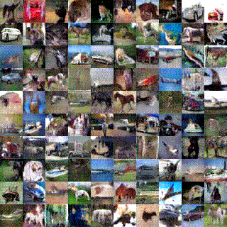
First, we execute the following cell and install “Chainer” and its GPU back end “CuPy”. If the “runtime type” of Colaboratory is GPU, you can run Chainer with GPU as a backend.
[2]:
!curl https://colab.chainer.org/install | sh -
Reading package lists... Done
Building dependency tree
Reading state information... Done
The following NEW packages will be installed:
libcusparse8.0 libnvrtc8.0 libnvtoolsext1
0 upgraded, 3 newly installed, 0 to remove and 0 not upgraded.
Need to get 28.9 MB of archives.
After this operation, 71.6 MB of additional disk space will be used.
Get:1 http://archive.ubuntu.com/ubuntu artful/multiverse amd64 libcusparse8.0 amd64 8.0.61-1 [22.6 MB]
Get:2 http://archive.ubuntu.com/ubuntu artful/multiverse amd64 libnvrtc8.0 amd64 8.0.61-1 [6,225 kB]
Get:3 http://archive.ubuntu.com/ubuntu artful/multiverse amd64 libnvtoolsext1 amd64 8.0.61-1 [32.2 kB]
Fetched 28.9 MB in 2s (14.4 MB/s)
Selecting previously unselected package libcusparse8.0:amd64.
(Reading database ... 18408 files and directories currently installed.)
Preparing to unpack .../libcusparse8.0_8.0.61-1_amd64.deb ...
Unpacking libcusparse8.0:amd64 (8.0.61-1) ...
Selecting previously unselected package libnvrtc8.0:amd64.
Preparing to unpack .../libnvrtc8.0_8.0.61-1_amd64.deb ...
Unpacking libnvrtc8.0:amd64 (8.0.61-1) ...
Selecting previously unselected package libnvtoolsext1:amd64.
Preparing to unpack .../libnvtoolsext1_8.0.61-1_amd64.deb ...
Unpacking libnvtoolsext1:amd64 (8.0.61-1) ...
Setting up libnvtoolsext1:amd64 (8.0.61-1) ...
Setting up libcusparse8.0:amd64 (8.0.61-1) ...
Setting up libnvrtc8.0:amd64 (8.0.61-1) ...
Processing triggers for libc-bin (2.26-0ubuntu2.1) ...
Let’s import the necessary modules, then check the version of Chainer, NumPy, CuPy, Cuda and other execution environments.
[ ]:
import os
import numpy as np
import chainer
from chainer import cuda
import chainer.functions as F
import chainer.links as L
from chainer import Variable
from chainer.training import extensions
chainer.print_runtime_info()
Chainer: 4.4.0
NumPy: 1.14.5
CuPy:
CuPy Version : 4.4.1
CUDA Root : None
CUDA Build Version : 8000
CUDA Driver Version : 9000
CUDA Runtime Version : 8000
cuDNN Build Version : 7102
cuDNN Version : 7102
NCCL Build Version : 2213
1. Setting parameters
Here we set the parameters for training.
n_epoch: Epoch number. How many times we pass through the whole training data.n_units: Number of units. How many hidden state vectors each Recursive Neural Network node has.batchsize: Batch size. How many train data we will input as a block when updating parameters.n_label: Number of labels. Number of classes to be identified. Since there are 5 labels this time,5.epoch_per_eval: How often to perform validation.is_test: IfTrue, we use a small dataset.gpu_id: GPU ID. The ID of the GPU to use. For Colaboratory it is good to use0.
[ ]:
# parameters
n_epoch = 100 # number of epochs
n_hidden = 100 # number of hidden units
batchsize = 50 # minibatch size
snapshot_interval = 10000 # number of iterations per snapshots
display_interval = 100 # number of iterations per display the status
gpu_id = 0
out_dir = 'result'
seed = 0 # random seed
2. Preparation of training data and iterator
In this notebook, we will use the training data which are preprocessed by chainer.datasets.get_cifar10.
From Wikipedia, it says
The CIFAR-10 dataset (Canadian Institute For Advanced Research) is a collection of images that are commonly used to train machine learning and computer vision algorithms. It is one of the most widely used datasets for machine learning research.The CIFAR-10 dataset contains 60,000 32x32 color images in 10 different classes. The 10 different classes represent airplanes, cars, birds, cats, deer, dogs, frogs, horses, ships, and trucks. There are 6,000 images of each class.
Let’s retrieve the CIFAR-10 dataset by using Chainer’s dataset utility function get_cifar10. CIFAR-10 is a set of small natural images. Each example is an RGB color image of size 32x32. In the original images, each component of pixels is represented by one-byte unsigned integer. This function scales the components to floating point values in the interval [0, scale].
[ ]:
# Load the CIFAR10 dataset if args.dataset is not specified
train, _ = chainer.datasets.get_cifar10(withlabel=False, scale=255.)
Downloading from https://www.cs.toronto.edu/~kriz/cifar-10-python.tar.gz...
[ ]:
train_iter = chainer.iterators.SerialIterator(train, batchsize)
3. Preparation of the model
Let’s define the network. We will create the model called DCGAN(Deep Convolutional GAN). As shown below, it is a model using CNN(Convolutional Neural Network) as its name suggests.
 cited from [1]
First, let’s define a network for the generator.
[ ]:
class Generator(chainer.Chain):
def __init__(self, n_hidden, bottom_width=4, ch=512, wscale=0.02):
super(Generator, self).__init__()
self.n_hidden = n_hidden
self.ch = ch
self.bottom_width = bottom_width
with self.init_scope():
w = chainer.initializers.Normal(wscale)
self.l0 = L.Linear(self.n_hidden, bottom_width * bottom_width * ch,
initialW=w)
self.dc1 = L.Deconvolution2D(ch, ch // 2, 4, 2, 1, initialW=w)
self.dc2 = L.Deconvolution2D(ch // 2, ch // 4, 4, 2, 1, initialW=w)
self.dc3 = L.Deconvolution2D(ch // 4, ch // 8, 4, 2, 1, initialW=w)
self.dc4 = L.Deconvolution2D(ch // 8, 3, 3, 1, 1, initialW=w)
self.bn0 = L.BatchNormalization(bottom_width * bottom_width * ch)
self.bn1 = L.BatchNormalization(ch // 2)
self.bn2 = L.BatchNormalization(ch // 4)
self.bn3 = L.BatchNormalization(ch // 8)
def make_hidden(self, batchsize):
return np.random.uniform(-1, 1, (batchsize, self.n_hidden, 1, 1)).astype(np.float32)
def __call__(self, z):
h = F.reshape(F.relu(self.bn0(self.l0(z))),
(len(z), self.ch, self.bottom_width, self.bottom_width))
h = F.relu(self.bn1(self.dc1(h)))
h = F.relu(self.bn2(self.dc2(h)))
h = F.relu(self.bn3(self.dc3(h)))
x = F.sigmoid(self.dc4(h))
return x
When we make a network in Chainer, we should follow some rules:
- Define a network class which inherits
Chain. - Make
chainer.links‘s instances in theinit_scope():of the initializer__init__. - Concatenate
chainer.links‘s instances withchainer.functionsto make the whole network.
If you are not familiar with constructing a new network, you can read this tutorial.
As we can see from the initializer __init__, the Generator uses the deconvolution layer Deconvolution2D and the batch normalization BatchNormalization. In __call__, each layer is concatenated by relu except the last layer.
Because the first argument of L.Deconvolution is the channel size of input and the second is the channel size of output, we can find that each layer halve the channel size. When we construct Generator with ch=1024, the network is same with the image above.
Note
Be careful when you concatenate a fully connected layer’s output and a convolutinal layer’s input. As we can see the 1st line of__call__, the output and input have to be concatenated with reshaping byreshape.
In addtion, let’s define a network for the discriminator.
[ ]:
class Discriminator(chainer.Chain):
def __init__(self, bottom_width=4, ch=512, wscale=0.02):
w = chainer.initializers.Normal(wscale)
super(Discriminator, self).__init__()
with self.init_scope():
self.c0_0 = L.Convolution2D(3, ch // 8, 3, 1, 1, initialW=w)
self.c0_1 = L.Convolution2D(ch // 8, ch // 4, 4, 2, 1, initialW=w)
self.c1_0 = L.Convolution2D(ch // 4, ch // 4, 3, 1, 1, initialW=w)
self.c1_1 = L.Convolution2D(ch // 4, ch // 2, 4, 2, 1, initialW=w)
self.c2_0 = L.Convolution2D(ch // 2, ch // 2, 3, 1, 1, initialW=w)
self.c2_1 = L.Convolution2D(ch // 2, ch // 1, 4, 2, 1, initialW=w)
self.c3_0 = L.Convolution2D(ch // 1, ch // 1, 3, 1, 1, initialW=w)
self.l4 = L.Linear(bottom_width * bottom_width * ch, 1, initialW=w)
self.bn0_1 = L.BatchNormalization(ch // 4, use_gamma=False)
self.bn1_0 = L.BatchNormalization(ch // 4, use_gamma=False)
self.bn1_1 = L.BatchNormalization(ch // 2, use_gamma=False)
self.bn2_0 = L.BatchNormalization(ch // 2, use_gamma=False)
self.bn2_1 = L.BatchNormalization(ch // 1, use_gamma=False)
self.bn3_0 = L.BatchNormalization(ch // 1, use_gamma=False)
def __call__(self, x):
h = add_noise(x)
h = F.leaky_relu(add_noise(self.c0_0(h)))
h = F.leaky_relu(add_noise(self.bn0_1(self.c0_1(h))))
h = F.leaky_relu(add_noise(self.bn1_0(self.c1_0(h))))
h = F.leaky_relu(add_noise(self.bn1_1(self.c1_1(h))))
h = F.leaky_relu(add_noise(self.bn2_0(self.c2_0(h))))
h = F.leaky_relu(add_noise(self.bn2_1(self.c2_1(h))))
h = F.leaky_relu(add_noise(self.bn3_0(self.c3_0(h))))
return self.l4(h)
The Discriminator network is almost same with the transposed network of the Generator. However, there are minor different points:
- Use
leaky_reluas activation functions - Deeper than
Generator - Add some noise when concatenating layers
[ ]:
def add_noise(h, sigma=0.2):
xp = cuda.get_array_module(h.data)
if chainer.config.train:
return h + sigma * xp.random.randn(*h.shape)
else:
return h
Let’s make the instances of the Generator and the Discriminator.
[ ]:
gen = Generator(n_hidden=n_hidden)
dis = Discriminator()
4. Preparing Optimizer
Next, let’s make optimizers for the models created above.
[ ]:
# Setup an optimizer
def make_optimizer(model, alpha=0.0002, beta1=0.5):
optimizer = chainer.optimizers.Adam(alpha=alpha, beta1=beta1)
optimizer.setup(model)
optimizer.add_hook(
chainer.optimizer_hooks.WeightDecay(0.0001), 'hook_dec')
return optimizer
[ ]:
opt_gen = make_optimizer(gen)
opt_dis = make_optimizer(dis)
5. Preparation and training of Updater · Trainer
The GAN need the two models: the generator and the discriminator. Usually, the default updaters pre-defined in Chainer take only one model. So, we need to define a custom updater for the GAN training.
The definition of DCGANUpdater is a little complicated. However, it just minimize the loss of the discriminator and that of the generator alternately. We will explain the way of updating the models.
As you can see in the class definiton, DCGANUpdater inherits StandardUpdater. In this case, almost all necessary functions are defined in StandardUpdater, we just override the functions of __init__ and update_core.
[ ]:
class DCGANUpdater(chainer.training.updaters.StandardUpdater):
def __init__(self, *args, **kwargs):
self.gen, self.dis = kwargs.pop('models')
super(DCGANUpdater, self).__init__(*args, **kwargs)
def loss_dis(self, dis, y_fake, y_real):
batchsize = len(y_fake)
L1 = F.sum(F.softplus(-y_real)) / batchsize
L2 = F.sum(F.softplus(y_fake)) / batchsize
loss = L1 + L2
chainer.report({'loss': loss}, dis)
return loss
def loss_gen(self, gen, y_fake):
batchsize = len(y_fake)
loss = F.sum(F.softplus(-y_fake)) / batchsize
chainer.report({'loss': loss}, gen)
return loss
def update_core(self):
gen_optimizer = self.get_optimizer('gen')
dis_optimizer = self.get_optimizer('dis')
batch = self.get_iterator('main').next()
x_real = Variable(self.converter(batch, self.device)) / 255.
xp = chainer.backends.cuda.get_array_module(x_real.data)
gen, dis = self.gen, self.dis
batchsize = len(batch)
y_real = dis(x_real)
z = Variable(xp.asarray(gen.make_hidden(batchsize)))
x_fake = gen(z)
y_fake = dis(x_fake)
dis_optimizer.update(self.loss_dis, dis, y_fake, y_real)
gen_optimizer.update(self.loss_gen, gen, y_fake)
In the intializer __init__, an addtional key word argument models is required as you can see the codes below. Also, we use key word arguments iterator, optimizer and device. Be careful for the optimizer. We needs not only two models but also two optimizers. So, we should input optimizer as dictionary {'gen': opt_gen, 'dis': opt_dis}. In the DCGANUpdater, you can access the iterator with self.get_iterator('main'). Also, you can access the optimizers with
self.get_optimizer('gen') and self.get_optimizer('dis').
In update_core, the two loss functions loss_dis and loss_gen are minimized by the optimizers. At first two lines, we access to the optimizers. Then, we generates next batch of training data by self.get_iterator('main').next(), and convert batch to x_real to make the training data suitable for self.device (e.g. GPU or CPU). After that, we minimize the loss functions with the optimizers.
[ ]:
updater = DCGANUpdater(
models=(gen, dis),
iterator=train_iter,
optimizer={
'gen': opt_gen, 'dis': opt_dis},
device=gpu_id)
trainer = chainer.training.Trainer(updater, (n_epoch, 'epoch'), out=out_dir)
[ ]:
from PIL import Image
import chainer.backends.cuda
def out_generated_image(gen, dis, rows, cols, seed, dst):
@chainer.training.make_extension()
def make_image(trainer):
np.random.seed(seed)
n_images = rows * cols
xp = gen.xp
z = Variable(xp.asarray(gen.make_hidden(n_images)))
with chainer.using_config('train', False):
x = gen(z)
x = chainer.backends.cuda.to_cpu(x.data)
np.random.seed()
x = np.asarray(np.clip(x * 255, 0.0, 255.0), dtype=np.uint8)
_, _, H, W = x.shape
x = x.reshape((rows, cols, 3, H, W))
x = x.transpose(0, 3, 1, 4, 2)
x = x.reshape((rows * H, cols * W, 3))
preview_dir = '{}/preview'.format(dst)
preview_path = preview_dir +\
'/image{:0>8}.png'.format(trainer.updater.iteration)
if not os.path.exists(preview_dir):
os.makedirs(preview_dir)
Image.fromarray(x).save(preview_path)
return make_image
[ ]:
snapshot_interval = (snapshot_interval, 'iteration')
display_interval = (display_interval, 'iteration')
trainer.extend(
extensions.snapshot(filename='snapshot_iter_{.updater.iteration}.npz'),
trigger=snapshot_interval)
trainer.extend(extensions.snapshot_object(
gen, 'gen_iter_{.updater.iteration}.npz'), trigger=snapshot_interval)
trainer.extend(extensions.snapshot_object(
dis, 'dis_iter_{.updater.iteration}.npz'), trigger=snapshot_interval)
trainer.extend(extensions.LogReport(trigger=display_interval))
trainer.extend(extensions.PrintReport([
'epoch', 'iteration', 'gen/loss', 'dis/loss',
]), trigger=display_interval)
trainer.extend(extensions.ProgressBar(update_interval=100))
trainer.extend(
out_generated_image(
gen, dis,
10, 10, seed, out_dir),
trigger=snapshot_interval)
[ ]:
# Run the training
trainer.run()
6. Checking the performance with test data
[ ]:
%%bash
ls result/preview
image00010000.png
image00020000.png
image00030000.png
image00040000.png
image00050000.png
image00060000.png
image00070000.png
image00080000.png
image00090000.png
image00100000.png
[ ]:
from IPython.display import Image, display_png
import glob
image_files = sorted(glob.glob(out_dir + '/preview/*.png'))
[ ]:
display_png(Image(image_files[0])) # first snapshot

[ ]:
display_png(Image(image_files[-1])) # last snapshot

Reference
[1] [Unsupervised Representation Learning with Deep Convolutional Generative Adversarial Networks](https://arxiv.org/abs/1511.06434)
Sentiment Analisys with Recursive Neural Network
Note: This notebook is created from chainer/examples/sentiment. If you want to run it as script, please refer to the above link.
In this notebook, we will analysys the sentiment of the documents by using Recursive Neural Network.
First, we execute the following cell and install “Chainer” and its GPU back end “CuPy”. If the “runtime type” of Colaboratory is GPU, you can run Chainer with GPU as a backend.
[1]:
!curl https://colab.chainer.org/install | sh -
Reading package lists... Done
Building dependency tree
Reading state information... Done
The following NEW packages will be installed:
libcusparse8.0 libnvrtc8.0 libnvtoolsext1
0 upgraded, 3 newly installed, 0 to remove and 0 not upgraded.
Need to get 28.9 MB of archives.
After this operation, 71.6 MB of additional disk space will be used.
Get:1 http://archive.ubuntu.com/ubuntu artful/multiverse amd64 libcusparse8.0 amd64 8.0.61-1 [22.6 MB]
Get:2 http://archive.ubuntu.com/ubuntu artful/multiverse amd64 libnvrtc8.0 amd64 8.0.61-1 [6,225 kB]
Get:3 http://archive.ubuntu.com/ubuntu artful/multiverse amd64 libnvtoolsext1 amd64 8.0.61-1 [32.2 kB]
Fetched 28.9 MB in 2s (10.4 MB/s)
78Selecting previously unselected package libcusparse8.0:amd64.
(Reading database ... 18298 files and directories currently installed.)
Preparing to unpack .../libcusparse8.0_8.0.61-1_amd64.deb ...
7Progress: [ 0%] [..........................................................] 87Progress: [ 6%] [###.......................................................] 8Unpacking libcusparse8.0:amd64 (8.0.61-1) ...
7Progress: [ 12%] [#######...................................................] 87Progress: [ 18%] [##########................................................] 8Selecting previously unselected package libnvrtc8.0:amd64.
Preparing to unpack .../libnvrtc8.0_8.0.61-1_amd64.deb ...
7Progress: [ 25%] [##############............................................] 8Unpacking libnvrtc8.0:amd64 (8.0.61-1) ...
7Progress: [ 31%] [##################........................................] 87Progress: [ 37%] [#####################.....................................] 8Selecting previously unselected package libnvtoolsext1:amd64.
Preparing to unpack .../libnvtoolsext1_8.0.61-1_amd64.deb ...
7Progress: [ 43%] [#########################.................................] 8Unpacking libnvtoolsext1:amd64 (8.0.61-1) ...
7Progress: [ 50%] [#############################.............................] 87Progress: [ 56%] [################################..........................] 8Setting up libnvtoolsext1:amd64 (8.0.61-1) ...
7Progress: [ 62%] [####################################......................] 87Progress: [ 68%] [#######################################...................] 8Setting up libcusparse8.0:amd64 (8.0.61-1) ...
7Progress: [ 75%] [###########################################...............] 87Progress: [ 81%] [###############################################...........] 8Setting up libnvrtc8.0:amd64 (8.0.61-1) ...
7Progress: [ 87%] [##################################################........] 87Progress: [ 93%] [######################################################....] 8Processing triggers for libc-bin (2.26-0ubuntu2.1) ...
78
Let’s import the necessary modules, then check the version of Chainer, NumPy, CuPy, Cuda and other execution environments.
[12]:
import collections
import numpy as np
import chainer
from chainer import cuda
import chainer.functions as F
import chainer.links as L
from chainer.training import extensions
from chainer import reporter
chainer.print_runtime_info()
Chainer: 4.1.0
NumPy: 1.14.3
CuPy:
CuPy Version : 4.1.0
CUDA Root : None
CUDA Build Version : 8000
CUDA Driver Version : 9000
CUDA Runtime Version : 8000
cuDNN Build Version : 7102
cuDNN Version : 7102
NCCL Build Version : 2104
1. Preparation of training data
In this notebook, we will use the training data which are preprocessed by chainer/examples/sentiment/download.py. Let’s run the following cells, download the necessary training data and unzip it.
[ ]:
# download.py
import os.path
from six.moves.urllib import request
import zipfile
request.urlretrieve(
'https://nlp.stanford.edu/sentiment/trainDevTestTrees_PTB.zip',
'trainDevTestTrees_PTB.zip')
zf = zipfile.ZipFile('trainDevTestTrees_PTB.zip')
for name in zf.namelist():
(dirname, filename) = os.path.split(name)
if not filename == '':
zf.extract(name, '.')
Let’s execute the following command and check if the training data have been prepared.
dev.txt test.txt train.txt
It will be OK if the above output is displayed.
[14]:
!ls trees
dev.txt test.txt train.txt
Let’s look at the first line of test.txt and see how each sample is written.
[15]:
!head trees/dev.txt -n1
(3 (2 It) (4 (4 (2 's) (4 (3 (2 a) (4 (3 lovely) (2 film))) (3 (2 with) (4 (3 (3 lovely) (2 performances)) (2 (2 by) (2 (2 (2 Buy) (2 and)) (2 Accorsi))))))) (2 .)))
As displayed above, each sample is defined by a tree structure.
The tree structure is recursively defined as (value, node), and the class label for node is value.
The class labels represent 1(really negative), 2(negative), 3(neutral), 4(positive), and 5(really positive), respectively.
The representation of the one sample is shown below.
2. Setting parameters
Here we set the parameters for training. * n_epoch: Epoch number. How many times we pass through the whole training data. * n_units: Number of units. How many hidden state vectors each Recursive Neural Network node has. * batchsize: Batch size. How many train data we will input as a block when updating parameters. * n_label: Number of labels. Number of classes to be identified. Since there are 5 labels this time, 5. * epoch_per_eval: How often to perform validation.
* is_test: If True, we use a small dataset. * gpu_id: GPU ID. The ID of the GPU to use. For Colaboratory it is good to use 0.
[ ]:
# parameters
n_epoch = 100 # number of epochs
n_units = 30 # number of units per layer
batchsize = 25 # minibatch size
n_label = 5 # number of labels
epoch_per_eval = 5 # number of epochs per evaluation
is_test = True
gpu_id = 0
if is_test:
max_size = 10
else:
max_size = None
3. Preparing the iterator
Let’s read the dataset used for training, validation, test and create an Iterator.
First, we convert each sample represented by str type to a tree structure data represented by a dictionary type.
We will tokenize the string with read_corpus implemented by the parser SexpParser. After that, we convert each tokenized sample to a tree structure data by convert_tree. By doing like this, it is possible to express a label as int, a node as a two-element tuple, and a tree structure as a dictionary, making it a more manageable data structure than the original string.
[ ]:
# data.py
import codecs
import re
class SexpParser(object):
def __init__(self, line):
self.tokens = re.findall(r'\(|\)|[^\(\) ]+', line)
self.pos = 0
def parse(self):
assert self.pos < len(self.tokens)
token = self.tokens[self.pos]
assert token != ')'
self.pos += 1
if token == '(':
children = []
while True:
assert self.pos < len(self.tokens)
if self.tokens[self.pos] == ')':
self.pos += 1
break
else:
children.append(self.parse())
return children
else:
return token
def read_corpus(path, max_size):
with codecs.open(path, encoding='utf-8') as f:
trees = []
for line in f:
line = line.strip()
tree = SexpParser(line).parse()
trees.append(tree)
if max_size and len(trees) >= max_size:
break
return trees
def convert_tree(vocab, exp):
assert isinstance(exp, list) and (len(exp) == 2 or len(exp) == 3)
if len(exp) == 2:
label, leaf = exp
if leaf not in vocab:
vocab[leaf] = len(vocab)
return {'label': int(label), 'node': vocab[leaf]}
elif len(exp) == 3:
label, left, right = exp
node = (convert_tree(vocab, left), convert_tree(vocab, right))
return {'label': int(label), 'node': node}
Let’s use read_corpus () and convert_tree () to create an iterator.
[ ]:
vocab = {}
train_data = [convert_tree(vocab, tree)
for tree in read_corpus('trees/train.txt', max_size)]
train_iter = chainer.iterators.SerialIterator(train_data, batchsize)
validation_data = [convert_tree(vocab, tree)
for tree in read_corpus('trees/dev.txt', max_size)]
validation_iter = chainer.iterators.SerialIterator(validation_data, batchsize,
repeat=False, shuffle=False)
test_data = [convert_tree(vocab, tree)
for tree in read_corpus('trees/test.txt', max_size)]
Let’s try to display the first element of test_data. It is represented by the following tree structure, lable expresses the score of that node, and the numerical value of the leaf node corresponds to the word id in the dictionary vocab.
[19]:
print(test_data[0])
{'label': 2, 'node': ({'label': 3, 'node': ({'label': 3, 'node': 252}, {'label': 2, 'node': 71})}, {'label': 1, 'node': ({'label': 1, 'node': 253}, {'label': 2, 'node': 254})})}
4. Preparing the model
Let’s define the network.
We traverse each node of the tree structure data by traverse and calculate the loss loss of the whole tree. The implementation of traverse is a recursive call, which will traverse child nodes in turn. (It is a common implementation when treating tree structure data!)
First, we calculate the hidden state vector v. In the case of a leaf node, we obtain a hidden state vector stored in embed by model.leaf(word) from word idword. In the case of an intermediate node, the hidden vector is calculated with the hidden state vector left and right of the child nodes by v = model.node(left, right).
loss += F.softmax_cross_entropy(y, t) adds the loss of the current node to the loss of the child node, then returns loss to the parent node by return loss, v.
After the line loss += F.softmax_cross_entropy(y, t), there are some lines for logging accuracy and etc. But it is not necessary for the model definition itself.
[ ]:
class RecursiveNet(chainer.Chain):
def traverse(self, node, evaluate=None, root=True):
if isinstance(node['node'], int):
# leaf node
word = self.xp.array([node['node']], np.int32)
loss = 0
v = model.leaf(word)
else:
# internal node
left_node, right_node = node['node']
left_loss, left = self.traverse(left_node, evaluate=evaluate, root=False)
right_loss, right = self.traverse(right_node, evaluate=evaluate, root=False)
v = model.node(left, right)
loss = left_loss + right_loss
y = model.label(v)
label = self.xp.array([node['label']], np.int32)
t = chainer.Variable(label)
loss += F.softmax_cross_entropy(y, t)
predict = cuda.to_cpu(y.data.argmax(1))
if predict[0] == node['label']:
evaluate['correct_node'] += 1
evaluate['total_node'] += 1
if root:
if predict[0] == node['label']:
evaluate['correct_root'] += 1
evaluate['total_root'] += 1
return loss, v
def __init__(self, n_vocab, n_units):
super(RecursiveNet, self).__init__()
with self.init_scope():
self.embed = L.EmbedID(n_vocab, n_units)
self.l = L.Linear(n_units * 2, n_units)
self.w = L.Linear(n_units, n_label)
def leaf(self, x):
return self.embed(x)
def node(self, left, right):
return F.tanh(self.l(F.concat((left, right))))
def label(self, v):
return self.w(v)
def __call__(self, x):
accum_loss = 0.0
result = collections.defaultdict(lambda: 0)
for tree in x:
loss, _ = self.traverse(tree, evaluate=result)
accum_loss += loss
reporter.report({'loss': accum_loss}, self)
reporter.report({'total': result['total_node']}, self)
reporter.report({'correct': result['correct_node']}, self)
return accum_loss
One attention to the implementation of __call__.
x passed to __call__ is mini-batched input data and contains samples s_n like [s_1, s_2, ..., s_N].
In a network such as Convolutional Network used for image recognition, it is possible to perform parallel calculation collectively for mini batch x. However, in the case of a tree-structured network like this one, it is difficult to compute parallel because of the following reasons.
- Data length varies depending on samples.
- The order of calculation for each sample is different.
So, the implementation is to calculate each sample and finally summarize the results.
Note: Actually, you can perform parallel calculation of mini batch in Recursive Neural Network by using stack. Since it is published in the latter part of notebook as (Advanced), please refer to it.
[ ]:
model = RecursiveNet(len(vocab), n_units)
if gpu_id >= 0:
model.to_gpu()
# Setup optimizer
optimizer = chainer.optimizers.AdaGrad(lr=0.1)
optimizer.setup(model)
optimizer.add_hook(chainer.optimizer_hooks.WeightDecay(0.0001))
5. Preparation and training of Updater · Trainer
As usual, we define an updater and a trainer to train the model. This time, I do not use L.Classifier and calculate the accuracy accuracy by myself. You can easily implement it using extensions.MicroAverage. For details, please refer to chainer.training.extensions.MicroAverage.
[22]:
def _convert(batch, device):
return batch
updater = chainer.training.StandardUpdater(
train_iter, optimizer, device=gpu_id, converter=_convert)
trainer = chainer.training.Trainer(updater, (n_epoch, 'epoch'))
trainer.extend(
extensions.Evaluator(validation_iter, model, device=gpu_id, converter=_convert),
trigger=(epoch_per_eval, 'epoch'))
trainer.extend(extensions.LogReport())
trainer.extend(extensions.MicroAverage(
'main/correct', 'main/total', 'main/accuracy'))
trainer.extend(extensions.MicroAverage(
'validation/main/correct', 'validation/main/total',
'validation/main/accuracy'))
trainer.extend(extensions.PrintReport(
['epoch', 'main/loss', 'validation/main/loss',
'main/accuracy', 'validation/main/accuracy', 'elapsed_time']))
trainer.run()
epoch main/loss validation/main/loss main/accuracy validation/main/accuracy elapsed_time
1 1707.8 0.155405 14.6668
2 586.467 556.419 0.497748 0.396175 17.3996
3 421.267 0.657658 19.3942
4 320.414 628.025 0.772523 0.42623 22.2462
5 399.621 0.704955 24.208
6 318.544 595.03 0.786036 0.420765 27.0585
7 231.529 0.880631 29.0178
8 160.546 628.959 0.916667 0.431694 31.7562
9 122.076 0.957207 33.8269
10 93.6623 669.898 0.975225 0.445355 36.5802
11 74.2366 0.986486 38.5855
12 60.2297 701.062 0.990991 0.448087 41.4308
13 49.7152 0.997748 43.414
14 41.633 724.893 0.997748 0.453552 46.1698
15 35.3564 0.997748 48.1999
16 30.402 744.493 1 0.448087 50.9842
17 26.4137 1 53.0605
18 23.188 760.43 1 0.459016 55.7924
19 20.5913 1 57.7479
20 18.4666 773.808 1 0.461749 60.5636
21 16.698 1 62.52
22 15.2066 785.205 1 0.461749 65.2603
23 13.9351 1 67.3052
24 12.8404 794.963 1 0.461749 70.0323
25 11.8897 1 71.9788
26 11.0575 803.388 1 0.459016 74.7653
27 10.3237 1 76.7485
28 9.67249 810.727 1 0.472678 79.4539
29 9.09113 1 81.4813
30 8.56935 817.176 1 0.480874 84.1942
31 8.09874 1 86.2475
32 7.6724 822.889 1 0.480874 88.956
33 7.2846 1 90.9035
34 6.93052 827.989 1 0.480874 93.6949
35 6.60615 1 95.6557
36 6.30805 832.574 1 0.486339 98.4233
37 6.03332 1 100.456
38 5.77941 836.724 1 0.486339 103.18
39 5.5442 1 105.129
40 5.32575 840.507 1 0.486339 107.954
6. Checking the performance with test data
[23]:
def evaluate(model, test_trees):
result = collections.defaultdict(lambda: 0)
with chainer.using_config('train', False), chainer.no_backprop_mode():
for tree in test_trees:
model.traverse(tree, evaluate=result)
acc_node = 100.0 * result['correct_node'] / result['total_node']
acc_root = 100.0 * result['correct_root'] / result['total_root']
print(' Node accuracy: {0:.2f} %% ({1:,d}/{2:,d})'.format(
acc_node, result['correct_node'], result['total_node']))
print(' Root accuracy: {0:.2f} %% ({1:,d}/{2:,d})'.format(
acc_root, result['correct_root'], result['total_root']))
print('Test evaluation')
evaluate(model, test_data)
Test evaluation
Node accuracy: 54.49 %% (170/312)
Root accuracy: 50.00 %% (5/10)
(Advanced) Mini-batching in Recursive Neural Network[1]
Recursive Neural Network is difficult to compute mini-batched data in parallel because of the following reasons.
- Data length varies depending on samples.
- The order of calculation for each sample is different.
However, using the stack, Recursive Neural Network can perform mini batch parallel calculation.
Preparation of Dataset, Iterator
First, we convert the recursive calculation of Recursive Neural Network to a serial calculation using a stack.
For each node of the tree structure dataset, numbers are assigned to each node in “returning order” as follows.
The returning order is a procedure of numbering nodes of a tree structure. It is a procedure of attaching a smaller number to all child nodes than the parent node. If you process nodes in descending order of numbers, you can trace the child nodes before the parent node.
[ ]:
def linearize_tree(vocab, root, xp=np):
# Left node indexes for all parent nodes
lefts = []
# Right node indexes for all parent nodes
rights = []
# Parent node indexes
dests = []
# All labels to predict for all parent nodes
labels = []
# All words of leaf nodes
words = []
# Leaf labels
leaf_labels = []
# Current leaf node index
leaf_index = [0]
def traverse_leaf(exp):
if len(exp) == 2:
label, leaf = exp
if leaf not in vocab:
vocab[leaf] = len(vocab)
words.append(vocab[leaf])
leaf_labels.append(int(label))
leaf_index[0] += 1
elif len(exp) == 3:
_, left, right = exp
traverse_leaf(left)
traverse_leaf(right)
traverse_leaf(root)
# Current internal node index
node_index = leaf_index
leaf_index = [0]
def traverse_node(exp):
if len(exp) == 2:
leaf_index[0] += 1
return leaf_index[0] - 1
elif len(exp) == 3:
label, left, right = exp
l = traverse_node(left)
r = traverse_node(right)
lefts.append(l)
rights.append(r)
dests.append(node_index[0])
labels.append(int(label))
node_index[0] += 1
return node_index[0] - 1
traverse_node(root)
assert len(lefts) == len(words) - 1
return {
'lefts': xp.array(lefts, 'i'),
'rights': xp.array(rights, 'i'),
'dests': xp.array(dests, 'i'),
'words': xp.array(words, 'i'),
'labels': xp.array(labels, 'i'),
'leaf_labels': xp.array(leaf_labels, 'i'),
}
[ ]:
xp = cuda.cupy if gpu_id >= 0 else np
vocab = {}
train_data = [linearize_tree(vocab, t, xp)
for t in read_corpus('trees/train.txt', max_size)]
train_iter = chainer.iterators.SerialIterator(train_data, batchsize)
validation_data = [linearize_tree(vocab, t, xp)
for t in read_corpus('trees/dev.txt', max_size)]
validation_iter = chainer.iterators.SerialIterator(
validation_data, batchsize, repeat=False, shuffle=False)
test_data = [linearize_tree(vocab, t, xp)
for t in read_corpus('trees/test.txt', max_size)]
Let’s try to display the first element of test_data.
lefts is the index of the left node for the dests parent node, rights is the index of the right node for the dests parent node, dests is the parent node’s index, dictionary contains word id,`labels has parent node label, and`` `leaf_labels`` contains dictionary of leaf node labels.
[26]:
print(test_data[0])
{'lefts': array([0, 2, 4], dtype=int32), 'rights': array([1, 3, 5], dtype=int32), 'dests': array([4, 5, 6], dtype=int32), 'words': array([252, 71, 253, 254], dtype=int32), 'labels': array([3, 1, 2], dtype=int32), 'leaf_labels': array([3, 2, 1, 2], dtype=int32)}
Definition of mini-batchable models
Recursive Neural Network has two operations: Operation A for computing an embedding vector for the leaf node. Operation B for computing the hidden state vector of the parent node from the hidden state vectors of the two child nodes.
For each sample, we assign index to each node in returning order. If you traverse the node in return order, you will find that operation A is performed on the leaf node and operation B is performed at the other nodes.
This operation can also be regarded as using a stack to scan a tree structure. A stack is a last-in, first-out data structure that allows you to do two things: a push operation to add data and a pop operation to get the last pushed data.
For operation A, push the calculation result to the stack. For operation B, pop two data and push the new calculation result.
When we parallelize the above operation, it is necessary to traverse nodes and perform operation A and operation B precisely because the tree structure is different for each sample. However, by using the stack, we can calculate different tree structures by simple repeating processing. Therefore, parallelization is possible.
[ ]:
from chainer import cuda
from chainer.utils import type_check
class ThinStackSet(chainer.Function):
"""Set values to a thin stack."""
def check_type_forward(self, in_types):
type_check.expect(in_types.size() == 3)
s_type, i_type, v_type = in_types
type_check.expect(
s_type.dtype.kind == 'f',
i_type.dtype.kind == 'i',
s_type.dtype == v_type.dtype,
s_type.ndim == 3,
i_type.ndim == 1,
v_type.ndim == 2,
s_type.shape[0] >= i_type.shape[0],
i_type.shape[0] == v_type.shape[0],
s_type.shape[2] == v_type.shape[1],
)
def forward(self, inputs):
xp = cuda.get_array_module(*inputs)
stack, indices, values = inputs
stack[xp.arange(len(indices)), indices] = values
return stack,
def backward(self, inputs, grads):
xp = cuda.get_array_module(*inputs)
_, indices, _ = inputs
g = grads[0]
gv = g[xp.arange(len(indices)), indices]
g[xp.arange(len(indices)), indices] = 0
return g, None, gv
def thin_stack_set(s, i, x):
return ThinStackSet()(s, i, x)
In addition, we use thin stack[2] instead of simple stack here.
Let the sentence length be \(I\) and the number of dimensions of the hidden vector be \(D\), the thin stack can efficiently use the memory by using the matrix of \((2I-1) \times D\).
In a normal stack, you need \(O(I^2 D)\) space computation, whereas thin stacks require \(O(ID)\).
It is realized by push operation thin_stack_set and pop operation thin_stack_get.
First of all, we define ThinStackSet and ThinStackGet which inherit chainer.Function.
ThinStackSet is literally a function to set values on the thin stack.
inputs in forward and backward can be broken down like stack, indices, values = inputs.
stack is shared by functions by setting it as a function argument in the thin stack itself.
Because chainer.Function does not have internal states inside, it handles stack externally by passing it as a function argument.
[ ]:
class ThinStackGet(chainer.Function):
def check_type_forward(self, in_types):
type_check.expect(in_types.size() == 2)
s_type, i_type = in_types
type_check.expect(
s_type.dtype.kind == 'f',
i_type.dtype.kind == 'i',
s_type.ndim == 3,
i_type.ndim == 1,
s_type.shape[0] >= i_type.shape[0],
)
def forward(self, inputs):
xp = cuda.get_array_module(*inputs)
stack, indices = inputs
return stack[xp.arange(len(indices)), indices], stack
def backward(self, inputs, grads):
xp = cuda.get_array_module(*inputs)
stack, indices = inputs
g, gs = grads
if gs is None:
gs = xp.zeros_like(stack)
if g is not None:
gs[xp.arange(len(indices)), indices] += g
return gs, None
def thin_stack_get(s, i):
return ThinStackGet()(s, i)
ThinStackGet is literally a function to retrieve values from the thin stack.
inputs in forward and backward can be broken down like stack, indices = inputs.
[ ]:
class ThinStackRecursiveNet(chainer.Chain):
def __init__(self, n_vocab, n_units, n_label):
super(ThinStackRecursiveNet, self).__init__(
embed=L.EmbedID(n_vocab, n_units),
l=L.Linear(n_units * 2, n_units),
w=L.Linear(n_units, n_label))
self.n_units = n_units
def leaf(self, x):
return self.embed(x)
def node(self, left, right):
return F.tanh(self.l(F.concat((left, right))))
def label(self, v):
return self.w(v)
def __call__(self, *inputs):
batch = len(inputs) // 6
lefts = inputs[0: batch]
rights = inputs[batch: batch * 2]
dests = inputs[batch * 2: batch * 3]
labels = inputs[batch * 3: batch * 4]
sequences = inputs[batch * 4: batch * 5]
leaf_labels = inputs[batch * 5: batch * 6]
inds = np.argsort([-len(l) for l in lefts])
# Sort all arrays in descending order and transpose them
lefts = F.transpose_sequence([lefts[i] for i in inds])
rights = F.transpose_sequence([rights[i] for i in inds])
dests = F.transpose_sequence([dests[i] for i in inds])
labels = F.transpose_sequence([labels[i] for i in inds])
sequences = F.transpose_sequence([sequences[i] for i in inds])
leaf_labels = F.transpose_sequence([leaf_labels[i] for i in inds])
batch = len(inds)
maxlen = len(sequences)
loss = 0
count = 0
correct = 0
# thin stack
stack = self.xp.zeros((batch, maxlen * 2, self.n_units), 'f')
# 葉ノードの隠れ状態ベクトルとlossを計算
for i, (word, label) in enumerate(zip(sequences, leaf_labels)):
batch = word.shape[0]
es = self.leaf(word)
ds = self.xp.full((batch,), i, 'i')
y = self.label(es)
loss += F.softmax_cross_entropy(y, label, normalize=False) * batch
count += batch
predict = self.xp.argmax(y.data, axis=1)
correct += (predict == label.data).sum()
stack = thin_stack_set(stack, ds, es)
# 中間ノードの隠れ状態ベクトルとlossを計算
for left, right, dest, label in zip(lefts, rights, dests, labels):
l, stack = thin_stack_get(stack, left)
r, stack = thin_stack_get(stack, right)
o = self.node(l, r)
y = self.label(o)
batch = l.shape[0]
loss += F.softmax_cross_entropy(y, label, normalize=False) * batch
count += batch
predict = self.xp.argmax(y.data, axis=1)
correct += (predict == label.data).sum()
stack = thin_stack_set(stack, dest, o)
loss /= count
reporter.report({'loss': loss}, self)
reporter.report({'total': count}, self)
reporter.report({'correct': correct}, self)
return loss
[ ]:
model = ThinStackRecursiveNet(len(vocab), n_units, n_label)
if gpu_id >= 0:
model.to_gpu()
optimizer = chainer.optimizers.AdaGrad(0.1)
optimizer.setup(model)
<chainer.optimizers.ada_grad.AdaGrad at 0x7f8a3c453710>
Preparation of Updater · Trainer and execution of training
Let’s train with the new model ThinStackRecursiveNet. Since you can now compute mini batches in parallel, you can see that training is faster.
[ ]:
def convert(batch, device):
if device is None:
def to_device(x):
return x
elif device < 0:
to_device = cuda.to_cpu
else:
def to_device(x):
return cuda.to_gpu(x, device, cuda.Stream.null)
return tuple(
[to_device(d['lefts']) for d in batch] +
[to_device(d['rights']) for d in batch] +
[to_device(d['dests']) for d in batch] +
[to_device(d['labels']) for d in batch] +
[to_device(d['words']) for d in batch] +
[to_device(d['leaf_labels']) for d in batch]
)
updater = chainer.training.StandardUpdater(
train_iter, optimizer, device=None, converter=convert)
trainer = chainer.training.Trainer(updater, (n_epoch, 'epoch'))
trainer.extend(
extensions.Evaluator(validation_iter, model, converter=convert, device=None),
trigger=(epoch_per_eval, 'epoch'))
trainer.extend(extensions.LogReport())
trainer.extend(extensions.MicroAverage(
'main/correct', 'main/total', 'main/accuracy'))
trainer.extend(extensions.MicroAverage(
'validation/main/correct', 'validation/main/total',
'validation/main/accuracy'))
trainer.extend(extensions.PrintReport(
['epoch', 'main/loss', 'validation/main/loss',
'main/accuracy', 'validation/main/accuracy', 'elapsed_time']))
trainer.run()
epoch main/loss validation/main/loss main/accuracy validation/main/accuracy elapsed_time
1 1.75582 0.268018 0.772637
2 1.0503 1.52234 0.63964 0.448087 1.74078
3 0.752925 0.743243 2.52495
4 1.21727 1.46956 0.745495 0.456284 3.49669
5 0.681582 0.817568 4.24974
6 0.477964 1.5514 0.880631 0.480874 5.22265
7 0.38437 0.916667 5.98324
8 0.30405 1.68066 0.923423 0.469945 6.94833
9 0.222884 0.959459 7.69772
10 0.175159 1.79104 0.977477 0.478142 8.67923
11 0.142888 0.97973 9.43108
12 0.118272 1.87948 0.986486 0.47541 10.4046
13 0.0991659 0.997748 11.1994
14 0.0841932 1.95415 0.997748 0.478142 12.1657
15 0.0723124 0.997748 12.9141
16 0.0627568 2.01682 0.997748 0.480874 13.8787
17 0.0549726 1 14.6336
18 0.04857 2.07107 1 0.478142 15.6061
19 0.0432675 1 16.3584
20 0.0388425 2.1181 1 0.480874 17.3297
21 0.035117 1 18.0761
22 0.0319522 2.15905 1 0.478142 19.0487
23 0.0292416 1 19.8416
24 0.0269031 2.1951 1 0.480874 20.8083
25 0.0248729 1 21.5566
26 0.0231 2.22721 1 0.483607 22.5304
27 0.0215427 1 23.2878
28 0.0201669 2.25614 1 0.486339 24.2565
29 0.018944 1 25.0171
30 0.017851 2.28247 1 0.480874 26.0063
31 0.0168687 1 26.7633
32 0.0159814 2.30664 1 0.483607 27.7331
33 0.0151763 1 28.5342
34 0.0144427 2.32898 1 0.483607 29.5039
35 0.0137716 1 30.257
36 0.0131555 2.34976 1 0.483607 31.2306
37 0.0125881 1 31.9842
38 0.0120638 2.3692 1 0.483607 32.9617
39 0.0115783 1 33.7175
40 0.0111272 2.38747 1 0.483607 34.6946
It got much faster!
Reference
[1] 深層学習による自然言語処理 (機械学習プロフェッショナルシリーズ)
[2] [A Fast Unified Model for Parsing and Sentence Understanding](http://nlp.stanford.edu/pubs/bowman2016spinn.pdf)
Word2Vec: Obtain word embeddings
0. Introduction
Word2vec is the tool for generating the distributed representation of words, which is proposed by Mikolov et al[1]. When the tool assigns a real-valued vector to each word, the closer the meanings of the words, the greater similarity the vectors will indicate.
Distributed representation means assigning a real-valued vector for each word and representing the word by the vector. When representing a word by distributed representation, we call the vector word embeddings. In this notebook, we aim at explaining how to get the word embeddings from Penn Tree Bank dataset.
Let’s think about what the meaning of word is. Since we are human, so we can understand that the words “animal” and “dog” are deeply related each other. But what information will Word2vec use to learn the vectors for words? The words “animal” and “dog” should have similar vectors, but the words “food” and “dog” should be far from each other. How to know the features of those words automatically?
1. Basic Idea
Word2vec learns the similarity of word meanings from simple information. It learns the representation of words from sentences. The core idea is based on the assumption that the meaning of a word is affected by the words around it. This idea follows distributional hypothesis[2].
The word we focus on to learn its representation is called “center word”, and the words around it are called “context words”. Depending on the window size C determines the number of context words which is considered.
Here, let’s see the algorithm by using an example sentence: “The cute cat jumps over the lazy dog.”
- All of the following figures consider “cat” as the center word.
- According to the window size
C, you can see that the number of context words is changed.
2. Main Algorithm
Word2vec, the tool for creating the word embeddings, is actually built with two models, which are called Skip-gram and CBoW.
To explain the models with the figures below, we will use the following symbols.
- \(|\mathcal{V}|\) : The size of vocabulary |
- \(D\) : The size of embedding vector |
- \({\bf v}_t\) : A one-hot center word vector |
- \(V_{\pm C}\) : A set of \(C\) context vectors around \({\bf v}_t\), namely, \(\{{\bf v}_{t+c}\}_{c=-C}^C \backslash {\bf v}_t\) |
- \({\bf l}_H\) : An embedding vector of an input word vector |
- \({\bf l}_O\) : An output vector of the network |
- \({\bf W}_H\) : The embedding matrix for inputs |
- \({\bf W}_O\) : The embedding matrix for outputs |
Note
Using negative sampling or hierarchical softmax for the loss function is very common, however, in this notebook, we will use the softmax over all words and skip the other variants for the sake of simplicity.
2.1 Skip-gram
This model learns to predict context words \(V_{t \pm C}\) when a center word \({\bf v}_t\) is given. In the model, each row of the embedding matrix for input \(W_H\) becomes a word embedding of each word.
When you input a center word \({\bf v}_t\) into the network, you can predict one of context words \(\hat{\bf v}_{t+i} \in V_{t \pm C}\) as follows:
- Calculate an embedding vector of the input center word vector: \({\bf l}_H = {\bf W}_H {\bf v}_t\)
- Calculate an output vector of the embedding vector: \({\bf l}_O = {\bf W}_O {\bf l}_H\)
- Calculate a probability vector of a context word: \(\hat{\bf v}_{t+i} = \text{softmax}({\bf l}_O)\)
Each element of the \(|\mathcal{V}|\)-dimensional vector \(\hat{\bf v}_{t+i}\) is a probability that a word in the vocabulary turns out to be a context word at position \(i\). So, the probability \(p({\bf v}_{t+i} \mid {\bf v}_t)\) can be estimated by a dot product of the one-hot vector \({\bf v}_{t+i}\) which represents the actual word at the position \(i\) and the output vector \(\hat{\bf v}_{t+i}\).
\(p({\bf v}_{t+i} \mid {\bf v}_t) = {\bf v}_{t+i}^T \hat{\bf v}_{t+i}\)
The loss function for all the context words \(V_{t \pm C}\) given a center word \({\bf v}_t\) is defined as following:
$
$
2.2 Continuous Bag of Words (CBoW)
This model learns to predict the center word \({\bf v}_t\) when context words \(V_{t \pm C}\) is given.
When you give a set of context words \(V_{t \pm C}\) to the network, you can estimate the probability of the center word \(\hat{v}_t\) as follows:
- Calculate a mean embedding vector over all context words: \({\bf l}_H = \frac{1}{2C} \sum_{V_{t \pm C}} {\bf W}_H {\bf v}_{t+i}\)
- Calculate an output vector: \({\bf l}_O = {\bf W}_O {\bf l}_H\)
- Calculate an probability vector: \(\hat{\bf v}_t = \text{softmax}({\bf l}_O)\)
Each element of \(\hat{\bf v}_t\) is a probability that a word in the vocabulary is considered as the center word. So, the prediction \(p({\bf v}_t \mid V_{t \pm C})\) can be calculated by \({\bf v}_t^T \hat{\bf v}_t\), where \({\bf v}_t\) denots the one-hot vector of the actual center word vector in the sentence from the dataset.
The loss function for the center word prediction is defined as follows:
$
$
3. Details of skip-gram
In this notebook, we mainly explain skip-gram model because
- It is easier to understand the algorithm than CBoW.
- Even if the number of words increases, the accuracy is largely maintained. So, it is more scalable.
So, let’s think about a concrete example of calculating skip-gram under this setup:
- The size of vocabulary \(|\mathcal{V}|\) is 10.
- The size of embedding vector \(D\) is 2.
- Center word is “dog”.
- Context word is “animal”.
Since there should be more than one context words, repeat the following process for each context word.
- The one-hot vector of “dog” is
[0 0 1 0 0 0 0 0 0 0]and you input it as the center word. - The third row of embedding matrix \({\bf W}_H\) is used for the word embedding of “dog” \({\bf l}_H\).
- Then multiply \({\bf W}_O\) with \({\bf l}_H\) to obtain the output vector \({\bf l}_O\)
- Give \({\bf l}_O\) to the softmax function to make it a predicted probability vector \(\hat{\bf v}_{t+c}\) for a context word at the position \(c\).
- Calculate the error between \(\hat{\bf v}_{t+c}\) and the one-hot vector of “animal”;
[1 0 0 0 0 0 0 0 0 0 0]. - Propagate the error back to the network to update the parameters.
4. Implementation of skip-gram in Chainer
There is an example of Word2vec in the official repository of Chainer, so we will explain how to implement skip-gram based on this: chainer/examples/word2vec
First, we execute the following cell and install “Chainer” and its GPU back end “CuPy”. If the “runtime type” of Colaboratory is GPU, you can run Chainer with GPU as a backend.
[1]:
!curl https://colab.chainer.org/install | sh -
Reading package lists... Done
Building dependency tree
Reading state information... Done
libcusparse8.0 is already the newest version (8.0.61-1).
libnvrtc8.0 is already the newest version (8.0.61-1).
libnvtoolsext1 is already the newest version (8.0.61-1).
0 upgraded, 0 newly installed, 0 to remove and 0 not upgraded.
4.1 Preparation
First, let’s import necessary packages:
[ ]:
import argparse
import collections
import numpy as np
import six
import chainer
from chainer import cuda
import chainer.functions as F
import chainer.initializers as I
import chainer.links as L
import chainer.optimizers as O
from chainer import reporter
from chainer import training
from chainer.training import extensions
4.2 Define a skip-gram model
Next, let’s define a network for skip-gram.
[ ]:
class SkipGram(chainer.Chain):
def __init__(self, n_vocab, n_units):
super().__init__()
with self.init_scope():
self.embed = L.EmbedID(
n_vocab, n_units, initialW=I.Uniform(1. / n_units))
self.out = L.Linear(n_units, n_vocab, initialW=0)
def __call__(self, x, context):
e = self.embed(context)
shape = e.shape
x = F.broadcast_to(x[:, None], (shape[0], shape[1]))
e = F.reshape(e, (shape[0] * shape[1], shape[2]))
x = F.reshape(x, (shape[0] * shape[1],))
center_predictions = self.out(e)
loss = F.softmax_cross_entropy(center_predictions, x)
reporter.report({'loss': loss}, self)
return loss
Note
- The weight matrix
self.embed.Wis the embbeding matrix for input vectorx. __call__takes the word ID of a center wordxand word IDs of context wordscontextsas inputs, and outputs the error calculated by the loss functionsoftmax_cross_entropy.- Note that the initial shape of
xandcontextsare(batch_size,)and(batch_size, n_context), respectively. - The
batch_sizemeans the size of mini-batch, andn_contextmeans the number of context words.
First, we obtain the embedding vectors of contexts by e = self.embed(contexts).
Then F.broadcast_to(x[:, None], (shape[0], shape[1])) performs broadcasting of x ((batch_size,)) to (batch_size, n_context) by copying the same value n_context time to fill the second axis, and then the broadcasted x is reshaped into 1-D vector (batchsize * n_context,) while e is reshaped to (batch_size * n_context, n_units).
In skip-gram model, predicting a context word from the center word is the same as predicting the center word from a context word because the center word is always a context word when considering the context word as a center word. So, we create batch_size * n_context center word predictions by applying self.out linear layer to the embedding vectors of context words. Then, calculate softmax cross entropy between the broadcasted center word ID x and the predictions.
4.3 Prepare dataset and iterator
Let’s retrieve the Penn Tree Bank (PTB) dataset by using Chainer’s dataset utility get_ptb_words() method.
[ ]:
train, val, _ = chainer.datasets.get_ptb_words()
n_vocab = max(train) + 1 # The minimum word ID is 0
Then define an iterator to make mini-batches that contain a set of center words with their context words.
[ ]:
class WindowIterator(chainer.dataset.Iterator):
def __init__(self, dataset, window, batch_size, repeat=True):
self.dataset = np.array(dataset, np.int32)
self.window = window
self.batch_size = batch_size
self._repeat = repeat
self.order = np.random.permutation(
len(dataset) - window * 2).astype(np.int32)
self.order += window
self.current_position = 0
self.epoch = 0
self.is_new_epoch = False
def __next__(self):
if not self._repeat and self.epoch > 0:
raise StopIteration
i = self.current_position
i_end = i + self.batch_size
position = self.order[i: i_end]
w = np.random.randint(self.window - 1) + 1
offset = np.concatenate([np.arange(-w, 0), np.arange(1, w + 1)])
pos = position[:, None] + offset[None, :]
context = self.dataset.take(pos)
center = self.dataset.take(position)
if i_end >= len(self.order):
np.random.shuffle(self.order)
self.epoch += 1
self.is_new_epoch = True
self.current_position = 0
else:
self.is_new_epoch = False
self.current_position = i_end
return center, context
@property
def epoch_detail(self):
return self.epoch + float(self.current_position) / len(self.order)
def serialize(self, serializer):
self.current_position = serializer('current_position',
self.current_position)
self.epoch = serializer('epoch', self.epoch)
self.is_new_epoch = serializer('is_new_epoch', self.is_new_epoch)
if self._order is not None:
serializer('_order', self._order)
def convert(batch, device):
center, context = batch
if device >= 0:
center = cuda.to_gpu(center)
context = cuda.to_gpu(context)
return center, context
- In the constructor, we create an array
self.orderwhich denotes shuffled indices of[window, window + 1, ..., len(dataset) - window - 1]in order to choose a center word randomly fromdatasetin a mini-batch. - The iterator definition
__next__returnsbatch_sizesets of center word and context words. - The code
self.order[i:i_end]returns the indices for a set of center words from the random-ordered arrayself.order. The center word IDscenterat the random indices are retrieved byself.dataset.take. np.concatenate([np.arange(-w, 0), np.arange(1, w + 1)])creates a set of offsets to retrieve context words from the dataset.- The code
position[:, None] + offset[None, :]generates the indices of context words for each center word index inposition. The context word IDscontextare retrieved byself.dataset.take.
4.4 Prepare model, optimizer, and updater
[ ]:
unit = 100 # number of hidden units
window = 5
batchsize = 1000
gpu = 0
# Instantiate model
model = SkipGram(n_vocab, unit)
if gpu >= 0:
model.to_gpu(gpu)
# Create optimizer
optimizer = O.Adam()
optimizer.setup(model)
# Create iterators for both train and val datasets
train_iter = WindowIterator(train, window, batchsize)
val_iter = WindowIterator(val, window, batchsize, repeat=False)
# Create updater
updater = training.StandardUpdater(
train_iter, optimizer, converter=convert, device=gpu)
4.5 Start training
[7]:
epoch = 100
trainer = training.Trainer(updater, (epoch, 'epoch'), out='word2vec_result')
trainer.extend(extensions.Evaluator(val_iter, model, converter=convert, device=gpu))
trainer.extend(extensions.LogReport())
trainer.extend(extensions.PrintReport(['epoch', 'main/loss', 'validation/main/loss', 'elapsed_time']))
trainer.run()
epoch main/loss validation/main/loss elapsed_time
1 6.87314 6.48688 54.154
2 6.44018 6.40645 107.352
3 6.35021 6.3558 159.544
4 6.28615 6.31679 212.612
5 6.23762 6.28779 266.059
6 6.19942 6.22658 319.874
7 6.15986 6.20715 372.798
8 6.13787 6.21461 426.456
9 6.10637 6.24927 479.725
10 6.08759 6.23192 532.966
11 6.06768 6.19332 586.339
12 6.04607 6.17291 639.295
13 6.0321 6.21226 692.67
14 6.02178 6.18489 746.599
15 6.00098 6.17341 799.408
16 5.99099 6.19581 852.966
17 5.97425 6.22275 905.819
18 5.95974 6.20495 958.404
19 5.96579 6.16532 1012.49
20 5.95292 6.21457 1066.24
21 5.93696 6.18441 1119.45
22 5.91804 6.20695 1171.98
23 5.93265 6.15757 1225.99
24 5.92238 6.17064 1279.85
25 5.9154 6.21545 1334.01
26 5.90538 6.1812 1387.68
27 5.8807 6.18523 1439.72
28 5.89009 6.19992 1492.67
29 5.8773 6.24146 1545.48
30 5.89217 6.21846 1599.79
31 5.88493 6.21654 1653.95
32 5.87784 6.18502 1707.45
33 5.88031 6.14161 1761.75
34 5.86278 6.22893 1815.29
35 5.83335 6.18966 1866.56
36 5.85978 6.24276 1920.18
37 5.85921 6.23888 1974.2
38 5.85195 6.19231 2027.92
39 5.8396 6.20542 2080.78
40 5.83745 6.27583 2133.37
41 5.85996 6.23596 2188
42 5.85743 6.17438 2242.4
43 5.84051 6.25449 2295.84
44 5.83023 6.30226 2348.84
45 5.84677 6.23473 2403.11
46 5.82406 6.27398 2456.11
47 5.82827 6.21509 2509.17
48 5.8253 6.23009 2562.15
49 5.83697 6.2564 2616.35
50 5.81998 6.29104 2669.38
51 5.82926 6.26068 2723.47
52 5.81457 6.30152 2776.36
53 5.82587 6.29581 2830.24
54 5.80614 6.30994 2882.85
55 5.8161 6.23224 2935.73
56 5.80867 6.26867 2988.48
57 5.79467 6.24508 3040.2
58 5.81687 6.24676 3093.57
59 5.82064 6.30236 3147.68
60 5.80855 6.30184 3200.75
61 5.81298 6.25173 3254.06
62 5.80753 6.32951 3307.42
63 5.82505 6.2472 3361.68
64 5.78396 6.28168 3413.14
65 5.80209 6.24962 3465.96
66 5.80107 6.326 3518.83
67 5.83765 6.28848 3574.57
68 5.7864 6.3506 3626.88
69 5.80329 6.30671 3679.82
70 5.80032 6.29277 3732.69
71 5.80647 6.30722 3786.21
72 5.8176 6.30046 3840.51
73 5.79912 6.35945 3893.81
74 5.80484 6.32439 3947.35
75 5.82065 6.29674 4002.03
76 5.80872 6.27921 4056.05
77 5.80891 6.28952 4110.1
78 5.79121 6.35363 4163.39
79 5.79161 6.32894 4216.34
80 5.78601 6.3255 4268.95
81 5.79062 6.29608 4321.73
82 5.7959 6.37235 4375.25
83 5.77828 6.31001 4427.44
84 5.7879 6.25628 4480.09
85 5.79297 6.29321 4533.27
86 5.79286 6.2725 4586.44
87 5.79388 6.36764 4639.82
88 5.79062 6.33841 4692.89
89 5.7879 6.31828 4745.68
90 5.81015 6.33247 4800.19
91 5.78858 6.37569 4853.31
92 5.7966 6.35733 4907.27
93 5.79814 6.34506 4961.09
94 5.81956 6.322 5016.65
95 5.81565 6.35974 5071.69
96 5.78953 6.37451 5125.02
97 5.7993 6.42065 5179.34
98 5.79129 6.37995 5232.89
99 5.76834 6.36254 5284.7
100 5.79829 6.3785 5338.93
[ ]:
vocab = chainer.datasets.get_ptb_words_vocabulary()
index2word = {wid: word for word, wid in six.iteritems(vocab)}
# Save the word2vec model
with open('word2vec.model', 'w') as f:
f.write('%d %d\n' % (len(index2word), unit))
w = cuda.to_cpu(model.embed.W.data)
for i, wi in enumerate(w):
v = ' '.join(map(str, wi))
f.write('%s %s\n' % (index2word[i], v))
4.6 Search the similar words
[ ]:
import numpy
import six
n_result = 5 # number of search result to show
with open('word2vec.model', 'r') as f:
ss = f.readline().split()
n_vocab, n_units = int(ss[0]), int(ss[1])
word2index = {}
index2word = {}
w = numpy.empty((n_vocab, n_units), dtype=numpy.float32)
for i, line in enumerate(f):
ss = line.split()
assert len(ss) == n_units + 1
word = ss[0]
word2index[word] = i
index2word[i] = word
w[i] = numpy.array([float(s) for s in ss[1:]], dtype=numpy.float32)
s = numpy.sqrt((w * w).sum(1))
w /= s.reshape((s.shape[0], 1)) # normalize
[ ]:
def search(query):
if query not in word2index:
print('"{0}" is not found'.format(query))
return
v = w[word2index[query]]
similarity = w.dot(v)
print('query: {}'.format(query))
count = 0
for i in (-similarity).argsort():
if numpy.isnan(similarity[i]):
continue
if index2word[i] == query:
continue
print('{0}: {1}'.format(index2word[i], similarity[i]))
count += 1
if count == n_result:
return
Search by “apple” word.
[23]:
query = "apple"
search(query)
query: apple
computer: 0.5457335710525513
compaq: 0.5068206191062927
microsoft: 0.4654524028301239
network: 0.42985647916793823
trotter: 0.42716777324676514
5. Reference
- [1] [Mikolov, Tomas; et al. “Efficient Estimation of Word Representations in Vector Space”. arXiv:1301.3781](https://arxiv.org/abs/1301.3781)
- [2] [Distributional Hypothesis](https://aclweb.org/aclwiki/Distributional_Hypothesis)
[ ]:
Other Examples
CuPy
1. Introduction
[ ]:
# Install CuPy and import as np !
!curl https://colab.chainer.org/install | sh -
import cupy as np
import numpy
Reading package lists... Done
Building dependency tree
Reading state information... Done
libcusparse8.0 is already the newest version (8.0.61-1).
libnvrtc8.0 is already the newest version (8.0.61-1).
libnvtoolsext1 is already the newest version (8.0.61-1).
0 upgraded, 0 newly installed, 0 to remove and 0 not upgraded.
Requirement already satisfied: cupy-cuda80==4.0.0b3 from https://github.com/kmaehashi/chainer-colab/releases/download/2018-02-06/cupy_cuda80-4.0.0b3-cp36-cp36m-linux_x86_64.whl in /usr/local/lib/python3.6/dist-packages
Requirement already satisfied: fastrlock>=0.3 in /usr/local/lib/python3.6/dist-packages (from cupy-cuda80==4.0.0b3)
Requirement already satisfied: six>=1.9.0 in /usr/local/lib/python3.6/dist-packages (from cupy-cuda80==4.0.0b3)
Requirement already satisfied: numpy>=1.9.0 in /usr/local/lib/python3.6/dist-packages (from cupy-cuda80==4.0.0b3)
[ ]:
class Regressor(object):
"""
Base class for regressors
"""
def fit(self, X, t, **kwargs):
"""
estimates parameters given training dataset
Parameters
----------
X : (sample_size, n_features) np.ndarray
training data input
t : (sample_size,) np.ndarray
training data target
"""
self._check_input(X)
self._check_target(t)
if hasattr(self, "_fit"):
self._fit(X, t, **kwargs)
else:
raise NotImplementedError
def predict(self, X, **kwargs):
"""
predict outputs of the model
Parameters
----------
X : (sample_size, n_features) np.ndarray
samples to predict their output
Returns
-------
y : (sample_size,) np.ndarray
prediction of each sample
"""
self._check_input(X)
if hasattr(self, "_predict"):
return self._predict(X, **kwargs)
else:
raise NotImplementedError
def _check_input(self, X):
if not isinstance(X, np.ndarray):
raise ValueError("X(input) is not np.ndarray")
if X.ndim != 2:
raise ValueError("X(input) is not two dimensional array")
if hasattr(self, "n_features") and self.n_features != np.size(X, 1):
raise ValueError(
"mismatch in dimension 1 of X(input) "
"(size {} is different from {})"
.format(np.size(X, 1), self.n_features)
)
def _check_target(self, t):
if not isinstance(t, np.ndarray):
raise ValueError("t(target) must be np.ndarray")
if t.ndim != 1:
raise ValueError("t(target) must be one dimenional array")
[ ]:
class LinearRegressor(Regressor):
"""
Linear regression model
y = X @ w
t ~ N(t|X @ w, var)
"""
def _fit(self, X, t):
self.w = np.linalg.pinv(X) @ t
self.var = np.mean(np.square(X @ self.w - t))
def _predict(self, X, return_std=False):
y = X @ self.w
if return_std:
y_std = np.sqrt(self.var) + np.zeros_like(y)
return y, y_std
return y
[ ]:
import matplotlib.pyplot as plt
%matplotlib inline
np.random.seed(1234)
1.1. Example: Polynomial Curve Fitting
[ ]:
def create_toy_data(func, sample_size, std):
x = np.linspace(0, 1, sample_size)
t = func(x) + np.random.normal(scale=std, size=x.shape)
return x, t
def func(x):
return np.sin(2 * 3.14 * x) # 3.14 should be np.pi
x_train, y_train = create_toy_data(func, 10, 0.25)
x_test = np.linspace(0, 1, 100)
y_test = func(x_test)
plt.scatter(x_train.get(), y_train.get(), facecolor="none", edgecolor="b", s=50, label="training data")
plt.plot(x_test.get(), y_test.get(), c="g", label="$\sin(2\pi x)$")
plt.legend()
plt.show()

[ ]:
import itertools
import functools
class PolynomialFeatures(object):
"""
polynomial features
transforms input array with polynomial features
Example
=======
x =
[[a, b],
[c, d]]
y = PolynomialFeatures(degree=2).transform(x)
y =
[[1, a, b, a^2, a * b, b^2],
[1, c, d, c^2, c * d, d^2]]
"""
def __init__(self, degree=2):
"""
construct polynomial features
Parameters
----------
degree : int
degree of polynomial
"""
assert isinstance(degree, int)
self.degree = degree
def transform(self, x):
"""
transforms input array with polynomial features
Parameters
----------
x : (sample_size, n) ndarray
input array
Returns
-------
output : (sample_size, 1 + nC1 + ... + nCd) ndarray
polynomial features
"""
if x.ndim == 1:
x = x[:, None]
x_t = x.transpose().get() # https://github.com/cupy/cupy/issues/1084
features = [numpy.ones(len(x))] # https://github.com/cupy/cupy/issues/1084
for degree in range(1, self.degree + 1):
for items in itertools.combinations_with_replacement(x_t, degree):
features.append(functools.reduce(lambda x, y: x * y, items))
features = numpy.array(features) # https://github.com/cupy/cupy/issues/1084
return np.asarray(features).transpose()
[ ]:
for i, degree in enumerate([0, 1, 3, 9]):
plt.subplot(2, 2, i + 1)
feature = PolynomialFeatures(degree)
X_train = feature.transform(x_train)
X_test = feature.transform(x_test)
model = LinearRegressor()
model.fit(X_train, y_train)
y = model.predict(X_test)
plt.scatter(x_train.get(), y_train.get(), facecolor="none", edgecolor="b", s=50, label="training data")
plt.plot(x_test.get(), y_test.get(), c="g", label="$\sin(2\pi x)$")
plt.plot(x_test.get(), y.get(), c="r", label="fitting")
plt.ylim(-1.5, 1.5)
plt.annotate("M={}".format(degree), xy=(-0.15, 1))
plt.legend(bbox_to_anchor=(1.05, 0.64), loc=2, borderaxespad=0.)
plt.show()

[ ]:
def rmse(a, b):
return np.sqrt(np.mean(np.square(a - b)))
training_errors = []
test_errors = []
for i in range(10):
feature = PolynomialFeatures(i)
X_train = feature.transform(x_train)
X_test = feature.transform(x_test)
model = LinearRegressor()
model.fit(X_train, y_train)
y = model.predict(X_test)
training_errors.append(rmse(model.predict(X_train), y_train))
test_errors.append(rmse(model.predict(X_test), y_test + np.random.normal(scale=0.25, size=len(y_test))))
plt.plot(training_errors, 'o-', mfc="none", mec="b", ms=10, c="b", label="Training")
plt.plot(test_errors, 'o-', mfc="none", mec="r", ms=10, c="r", label="Test")
plt.legend()
plt.xlabel("degree")
plt.ylabel("RMSE")
plt.show()

Regularization
[ ]:
class RidgeRegressor(Regressor):
"""
Ridge regression model
w* = argmin |t - X @ w| + a * |w|_2^2
"""
def __init__(self, alpha=1.):
self.alpha = alpha
def _fit(self, X, t):
eye = np.eye(np.size(X, 1))
self.w = np.linalg.solve(self.alpha * eye + X.T @ X, X.T @ t)
def _predict(self, X):
y = X @ self.w
return y
[ ]:
feature = PolynomialFeatures(9)
X_train = feature.transform(x_train)
X_test = feature.transform(x_test)
model = RidgeRegressor(alpha=1e-3)
model.fit(X_train, y_train)
y = model.predict(X_test)
y = model.predict(X_test)
plt.scatter(x_train.get(), y_train.get(), facecolor="none", edgecolor="b", s=50, label="training data")
plt.plot(x_test.get(), y_test.get(), c="g", label="$\sin(2\pi x)$")
plt.plot(x_test.get(), y.get(), c="r", label="fitting")
plt.ylim(-1.5, 1.5)
plt.legend()
plt.annotate("M=9", xy=(-0.15, 1))
plt.show()

[ ]:
class BayesianRegressor(Regressor):
"""
Bayesian regression model
w ~ N(w|0, alpha^(-1)I)
y = X @ w
t ~ N(t|X @ w, beta^(-1))
"""
def __init__(self, alpha=1., beta=1.):
self.alpha = alpha
self.beta = beta
self.w_mean = None
self.w_precision = None
def _fit(self, X, t):
if self.w_mean is not None:
mean_prev = self.w_mean
else:
mean_prev = np.zeros(np.size(X, 1))
if self.w_precision is not None:
precision_prev = self.w_precision
else:
precision_prev = self.alpha * np.eye(np.size(X, 1))
w_precision = precision_prev + self.beta * X.T @ X
w_mean = np.linalg.solve(
w_precision,
precision_prev @ mean_prev + self.beta * X.T @ t
)
self.w_mean = w_mean
self.w_precision = w_precision
self.w_cov = np.linalg.inv(self.w_precision)
def _predict(self, X, return_std=False, sample_size=None):
if isinstance(sample_size, int):
w_sample = np.random.multivariate_normal(
self.w_mean, self.w_cov, size=sample_size
)
y = X @ w_sample.T
return y
y = X @ self.w_mean
if return_std:
y_var = 1 / self.beta + np.sum(X @ self.w_cov * X, axis=1)
y_std = np.sqrt(y_var)
return y, y_std
return y
[ ]:
model = BayesianRegressor(alpha=2e-3, beta=2)
model.fit(X_train, y_train)
y, y_err = model.predict(X_test, return_std=True)
plt.scatter(x_train.get(), y_train.get(), facecolor="none", edgecolor="b", s=50, label="training data")
plt.plot(x_test.get(), y_test.get(), c="g", label="$\sin(2\pi x)$")
plt.plot(x_test.get(), y.get(), c="r", label="mean")
plt.fill_between(x_test.get(), (y - y_err).get(), (y + y_err).get(), color="pink", label="std.", alpha=0.5)
plt.xlim(-0.1, 1.1)
plt.ylim(-1.5, 1.5)
plt.annotate("M=9", xy=(0.8, 1))
plt.legend(bbox_to_anchor=(1.05, 1.), loc=2, borderaxespad=0.)
plt.show()
